Its about time pass

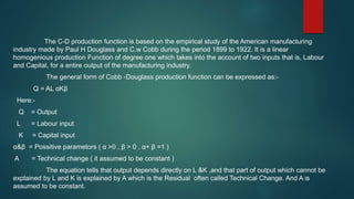
1. COBB-DOUGLAS
PRODUCTION FUNCTION

2. The C-D production function is based on the empirical study of the American manufacturing
industry made by Paul H Douglass and C.w Cobb during the period 1899 to 1922. It is a linear
homogenious production Function of degree one which takes into the account of two inputs that is, Labour
and Capital, for a entire output of the manufacturing industry.
The general form of Cobb -Douglass production function can be expressed as:-
Q = AL αKβ
Here:-
Q = Output
L = Labour input
K = Capital input
α&β = Possitive parametors ( α >0 , β > 0 , α+ β =1 )
A = Technical change ( it assumed to be constant )
The equation tells that output depends directly on L &K ,and that part of output which cannot be
explained by L and K is explained by A which is the Residual often called Technical Change. And A is
assumed to be constant.

3. Properties
The following are the important properties of Cobb-Douglass production
function:-
1.Constant Returns to Scale
C – D production function exhibits constant returns to scale . To prove it ,
let us increase the quantities of L & K by λ times and output must also
increased by λ times . Then the increased output (Q*) will be ;
Q* = λQ
 α+β=1 Constant returns to scale
 α+β>1 Increasing returns to scale
 α+β<1 Diminishing returns to scale

4. 2. The Average Product (AP) and Marginal Product (MP) of factors
The C-D production function tells that the AP & MP of factors is a function of the
ratio of the factors .
Q = ALαKβ
APL = A (K/L)β
APK = A (L/K)α
MPL = α A (K/L)β
MPK = β A (L/K )α
3. Marginal Rate of Substitution between Capital and Labour (MRS LK)
The MRS LK can be derived from the C-D production function.
MRS LK = ∂Q/∂L ÷ ∂Q /∂K

5. 4. Elasticity of factors substitution
The Elasticity of factors substitution of the C-D production function is equal to unity.
Its proof, the elasticity of substitution (es) between K&L is defined as;
σ = ( f1 × f2 )/(f12 × Q)
Here ;
 f1 =MPL
 f2 = MPK
 f12 = cross partial derivative of L& K
∂Q = ∂L × ∂K
σ = 1
when the elasticity of substitution is unity the production function is homogenious of
degree one. That is constant returns to scale

6.  5. Euler’s theorum
 The application of Euler’s theorum to distribution in an other
property of the C-D production function . If the production function
 Q = f(K/L) is homogenious of degree one , then according to Euler’s
theorum
 Q = L (∂Q/∂L) + K ( ∂Q/∂K )
 Apply the general form of C-D production function we get Q = Q

7.  6. Factor intensity
 In the C-D production function Q = ALαKβ , the factor intensity is
measured by the ratio ( α /β ). Higher the ratio , the production function is
more labour intensive and lower the ratio , the production function will be
capital intensive .
 7. Efficiency of production
 The coefficient ‘A’ in the C-D production function helps in
measuring the efficiency in the organisation of the factors of production. If
two firms have the same α , β , L and K but produce different quantities of
output , this difference may be due to the superior organisation of more
efficient firm as against the other. The more efficient firm will have a larger ‘
A ‘ than the other firm

8.  8. Multiplicative Function
 The C-D production function is a multiplicative function . It means that if an input
has zero value , the output will also be zero . This property highlights the fact that all
inputs are necessary for production in a firm.
 9. Output elasticity
 It can be defined as the proportionate change in output with a given change in
input . The output elasticity of L & K can be calculated with the help of C-D production
function :-
 Output elasticity of labour = ( ∂Q / ∂L ) ÷ ( L / Q )
 Output elasticity of capital = ( ∂Q / ∂K ) ÷ (K / Q )

9. Criticisms
 The C-D production function considers only two inputs , labour and capital
and neglects some important inputs like raw materials , which are used in
production.
 In the C-D production function , the problem of measurement of capital
arises because it takes only the quantity of capital available for production .
But the full use of the available capital can be made only in periods of
fullemployment. This is unrealistic situation.
 The C-D production function is criticised because it shows constant returns
to scale. But constant returns to scale are not an actuality , for either
increasing or decreasing returns to scale are applicable to production.

10.  The C-D production function is based on the assumption of substitutability
of factors and neglects the complimentarity of factors.
 This function is based on the assumption of perfect competitionin the
factor market which is unrealistic.
 One of the weakness of C-D production function is the aggregation
problem.

11. Importance
 The C-D production function has been used widely in empirical studies of manufacturing
industries and in inter-industry comparisons.
 It is used to determine the relative shares of labour and capital in total output. And it is
also used to prove Euler’s theorum.
 Its parametors α and β represents elasticity coefficients that are used for inter-sectoral
comparisons.
 This production function is linear homogenious of degree one which shows constant
returns to scale.
 If α + β >1 - increasing returns to scale
 α + β <1 - decreasing returns to scale
 This production function is more than two variables.

12. Conclusion
 Thus the practicability of the C-D production function in the
manufacturing industry is a doubtful proposition. This is not applicable to
agriculture where for intensive cultivation , increasing the quantity of inputs
will not raise output proportionately.

13. THANK YOU