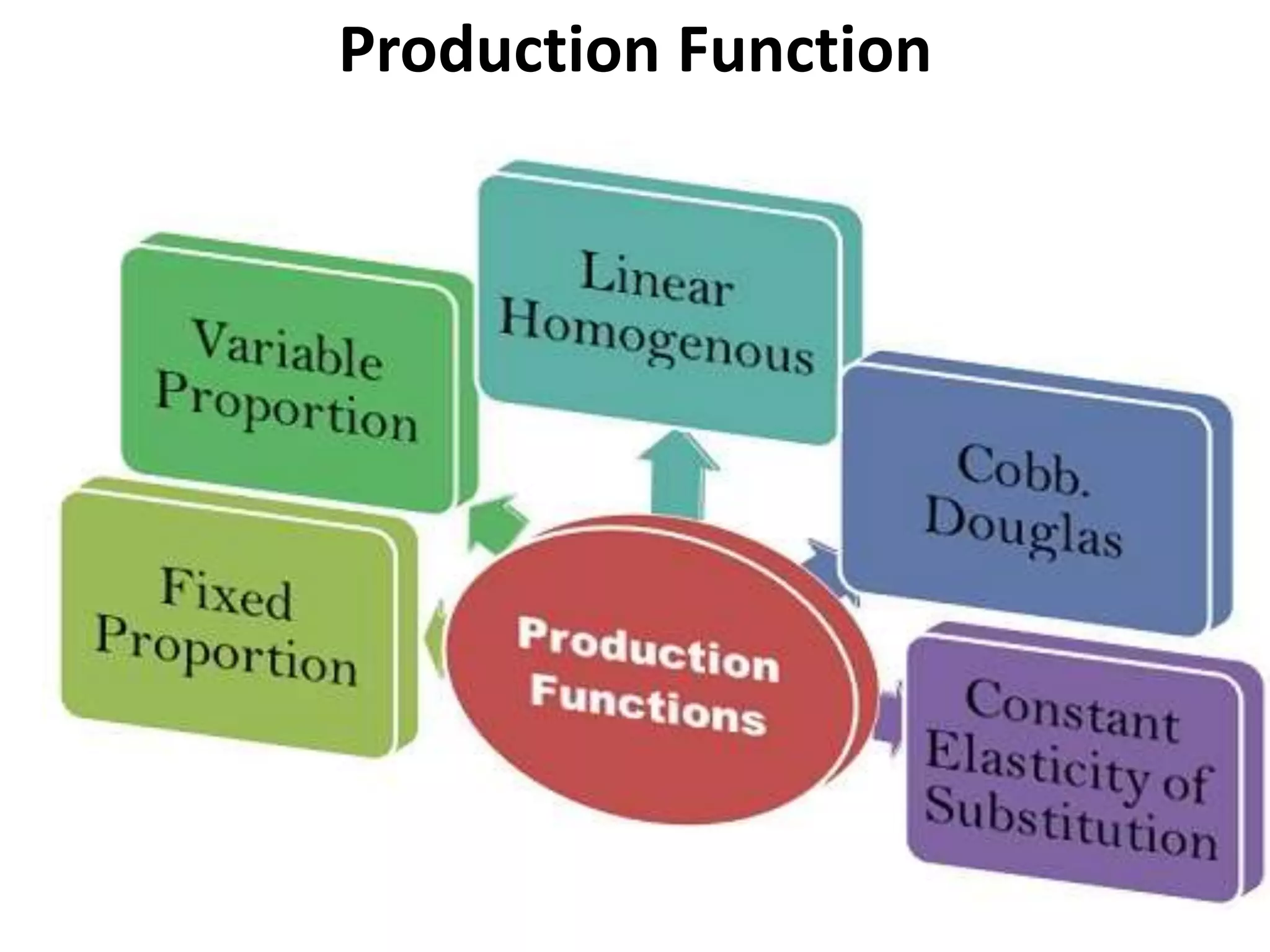
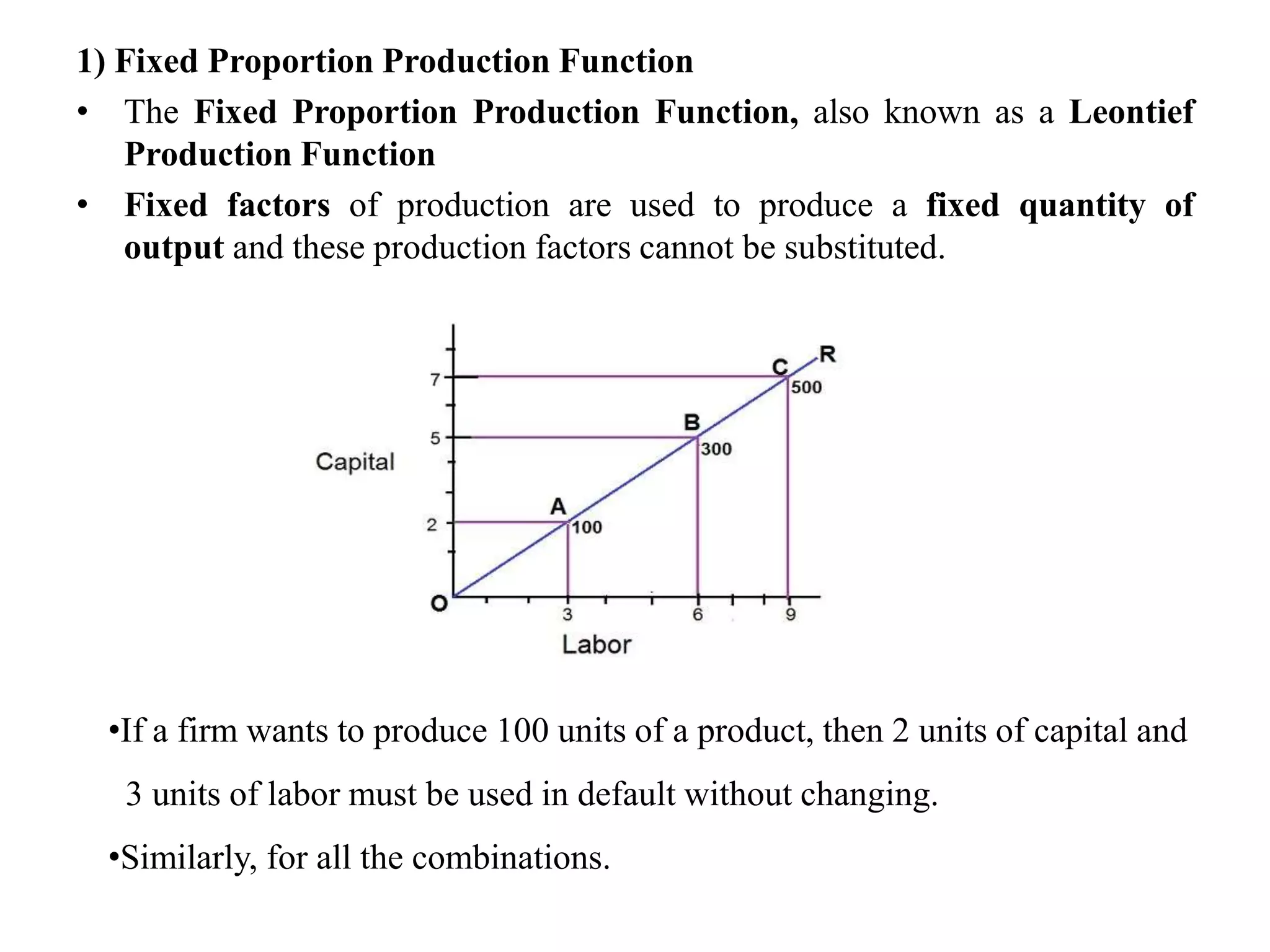
1) This document discusses various concepts related to production analysis including factors of production, production functions, laws of variable proportions, isoquants, marginal rate of technical substitution, and returns to scale. 2) The factors of production are land, labor, capital, and entrepreneurship. Production functions include fixed proportion, variable proportion, linear homogeneous, Cobb-Douglas, and constant elasticity of substitution. 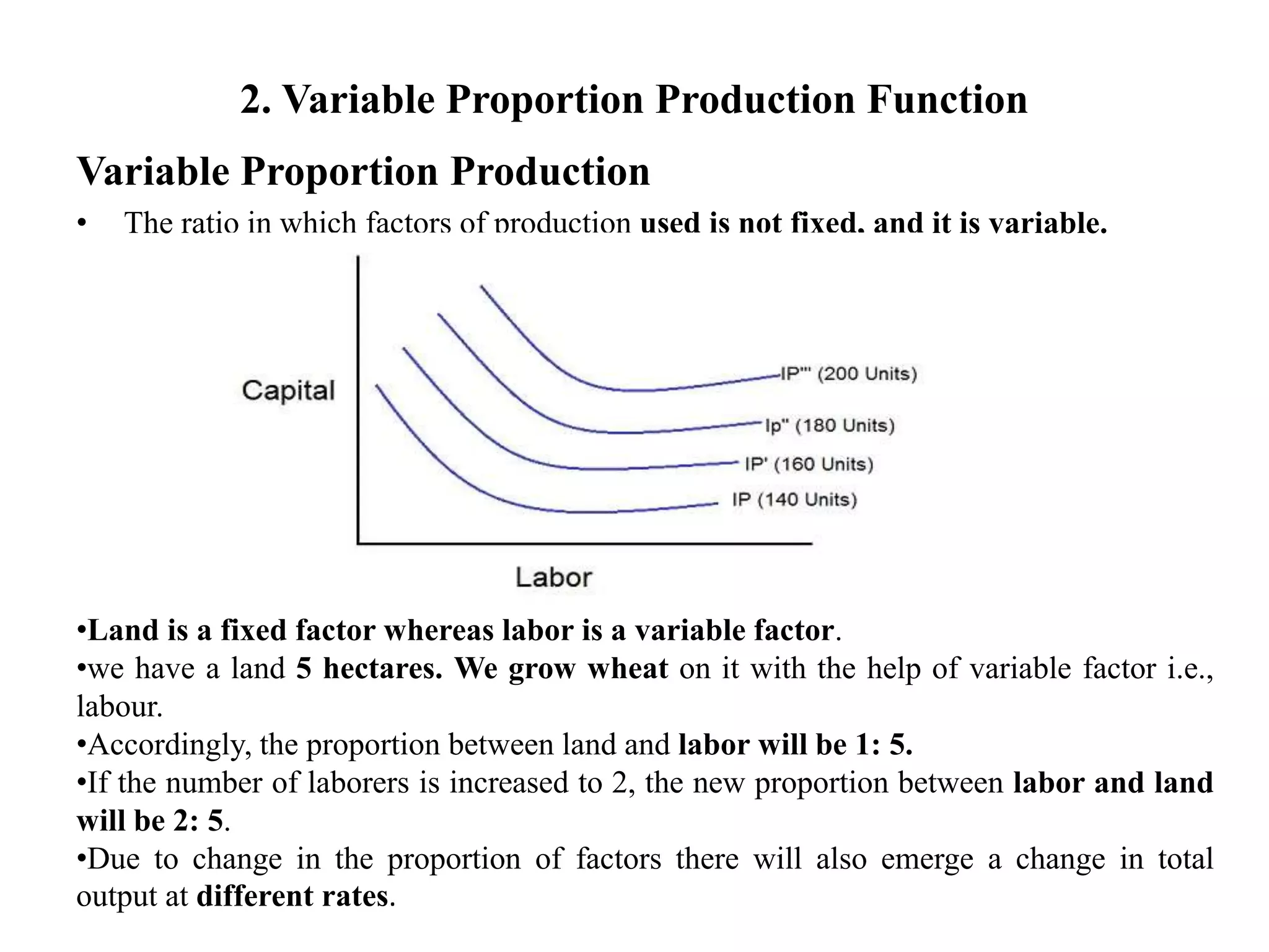3) The law of variable proportions explains how output increases at different rates as one variable input is increased while others stay fixed. Returns to scale refers to how output changes as all inputs change proportionately.

1. UNIT - 3
1) Production analysis
2) Factors of production-
3) Production function
4) Law of variable proportion
5) Isoquants
6) Marginal rate of technical substitutions
(MRS)
7) Law of Returns to scale
8) Comparisons between Returns to factors
and Returns to scale

2. Production analysis
• "Production is the creation of economic utility "- Ely
• Production is a process of transformation of the
factors of production into the economic goods.

5. Factor of Production
Land:
• Land includes all natural physical resources – e.g.
fertile farm land.
• Land is that factor of production which is freely
available from nature including forests, minerals,
fertility of soil, water, etc.

6. Labour:
• Labour is the human input into production.
• Including all those mental and physical activities
of man which are performed in order to earn
money.
• The services of a carpenter, black-smith,
weaver, teacher, lawyer and doctor, etc., are
called labour.

7. Capital:
• Capital: Capital is a man-made factor of production
used for investment in machines, tools, raw
materials, buildings, etc.
• Fixed capital includes investment in machinery,
equipment, new technology, factories and other
buildings
• Working capital is proposed to meet day to day
business needs.

8. Entrepreneurship/Organisation
• Entrepreneurship has been described as the "capacity and
willingness to develop, organize and manage a business
venture along with any of its risks to make a profit."
• Entrepreneurs will usually invest financial capital in a
business and take on the risks.
• Their main reward is the profit made from running the
business

9. Production Function

10. 1) Fixed Proportion Production Function
• The Fixed Proportion Production Function, also known as a Leontief
Production Function
• Fixed factors of production are used to produce a fixed quantity of
output and these production factors cannot be substituted.
•If a firm wants to produce 100 units of a product, then 2 units of capital and
3 units of labor must be used in default without changing.
•Similarly, for all the combinations.

11. 2. Variable Proportion Production Function
Variable Proportion Production
• The ratio in which factors of production used is not fixed, and it is variable.
•Land is a fixed factor whereas labor is a variable factor.
•we have a land 5 hectares. We grow wheat on it with the help of variable factor i.e.,
labour.
•Accordingly, the proportion between land and labor will be 1: 5.
•If the number of laborers is increased to 2, the new proportion between labor and land
will be 2: 5.
•Due to change in the proportion of factors there will also emerge a change in total
output at different rates.

12. 3.Linear Homogeneous Production Function
• Proportionate change in all the factors of production, the output also increases in the
same proportion. (if input doubled, output also gets doubled)
• In the case of a linear homogeneous production function, the expansion is always a straight
line through the origin.
• This means that the proportions between the factors used will always be the same provided
the factor prices remains constant

13. 4. Cobb-Douglas Production Function
• In 1928, Charles Cobb and Paul Douglas presented this model.
• The Cobb-Douglas production function represents the relationship
between two or more inputs - typically capital and labor - and the
number of outputs that can be produced.
• The concept associated with the Cobb-Douglas production function is
marginal product, which is the change in the output that results from
one additional unit of a single production factor with all other factors
held constant.
L-Labour
K-Capital
A- Total Factor productivity

14. Marginal product= (100-200)=100 units( derived as a result of increasing L1
to L2 and C1 to C2)

15. 5. Constant Elasticity of Substitution (CES)
Production Function
• The Constant Elasticity of Substitution Production Function or CES
implies, that any change in the input factors, results in the constant change
in the output.

16. • To produce 100 units of
output, ОС1, units of
capital and OL1 units of
labor are used.
• If the output were to be
doubled to 200, the
inputs of labor and capital
would have to be
doubled.
• ОС2 is exactly double of
ОС1 and of OL2 is double
of OL1.
• Similarly, if the output is
to be raised three-fold to
300, the units of labor
and capital will have to be
increased three-fold.

17. Law of variable proportion
• This law examines the input-output relation
when output is increased by varying the
quantity of one input.
Definitions:
“An increase in some inputs relative to other
fixed inputs will in a given state of technology
cause output to increase, but after a point the
extra output resulting from the same additions
of extra inputs will become less and less.”
Samuelson

18. Assumptions
1) Stable technology
If there is an enhancement in technology the
production function will move in the upward
direction.
2) Fixed Amount of Other Factors: there must be
some inputs whose quantity is kept fixed. The
law does not apply if all factors are
proportionately varied.
3) Possibility of Varying the Factor proportions:
The law does not apply if the factors must be used
in fixed proportions to yield a product.

19. Explanation of the Law

20. • Let us take the example of agriculture, where
land and labor are the only two factors of
production. By keeping the land as a
permanent factor, the production of variable
factor i.e., labor can be shown with the help
of the above table.

21. • The 3 Stages of the Law
• First Stage
• The first stage starts from point ‘O’ and ends up
to point F. At point F regular product is utmost
and is equal to marginal product. In this stage,
the total product becomes higher initially at
increasing rate up to point E. between ‘E’ and ‘F’
it becomes higher at diminishing rate. in the
same way, the marginal product also becomes
higher at first and reaches its utmost at point ‘H’.
it then begins to diminish and becomes equal to a
regular product at point T. In this stage, marginal
product surpasses regular product (MP > AP).

22. • 2) Second stage
• It begins from the point F. In this stage, the
total product becomes higher at diminishing
rate and is at its utmost at point ‘G’
correspondingly marginal product diminishes
rapidly and becomes ‘zero’ at point ‘C’. A
regular product is utmost at point ‘I’ and
thereafter it begins to decrease. In this stage,
marginal product is less than the regular
product (MP < AP).

23. 3) Third stage
• This stage begins beyond point ‘G’. Here total
product starts diminishing. The regular
product also declines. The marginal product
turns negative. Law of diminishing returns
firmly manifests itself. In this stage, no
company will produce anything. This is due to
the marginal product of the labour becomes
negative. The employer will endure losses by
employing more units of labourers. but, of the
three stages, a firm will like to produce up to
any given point in the second stage merely.

24. The 3 Stages of the Law of Variable Proportions

25. ISOQUANT
• The term Iso-quant or Iso-product is
composed of two words, Iso = equal, quant =
quantity or product = output.
• As isoquant curve can be defined as the locus
of points representing various combinations of
two inputs capital and labor yielding the same
output.

26. Definitions:
“Iso-product curve shows the different input
combinations that will produce a given
output.” Samuelson

27. Assumptions:
1. Two Factors of Production:
Only two factors are used to produce a commodity.
2. Divisible Factor:
Factors of production can be divided into small
parts.
3. Constant Technique:
Technique of production is constant or is known
before hand.

28. 4. Possibility of Technical Substitution:
The substitution between the two factors is
technically possible. That is, production
function is of ‘variable proportion’.(labour and
capital) type rather than fixed proportion
(land)
5. Efficient Combinations:
Under the given technique, factors of
production can be used with maximum
efficiency.

29. • The table 1 shows that the
five combinations of labour
units and units of capital
yield the same level of
output, i.e., 200 metres of
cloth.
• Thus, 200 metre cloth can be
produced by combining.
• (a) 1 units of labour and 15
units of capital
• (b) 2 units of labour and 11
units of capital
• (c) 3 units of labour and 8
units of capital
• (d) 4 units of labour and 6
units of capital
• (e) 5 units of labour and 5
units of capital

30. Iso-Product Curve:
The Fig. 1 shows the
various combinations of
labour and capital which
give the same amount of
output. A, B, C, D and E.

31. Marginal rate of technical substitution (MRTS)
• The rate at which one factor must be
decreased so that the same level of
productivity can be maintained when another
factor is increased.
• The MRTS reflects the give-and-take between
factors, such as capital and labor, that allow a
firm to maintain a constant output.

32. • The marginal rate of technical substitution
(MRTS) can be defined as, keeping constant
the total output, how much input 1 have to
decrease if input 2 increases by one extra unit.

33. Combination Labour Capital MRTSLK(∆K. ∆L) =
change in
capital:change in
labour
Output
1 5 9 — 100
2 10 6 3:5 100
3 15 4 2:5 100
4 20 3 1:5 100

34. • The above table shows that
in the second combination
to keep output constant at
100 units, the reduction of
3 units of capital requires
the addition of 5 units of
labour, MRTSLk= 3:5. In the
third combination, the loss
of 2 units of capital is
compensated for by 5 more
units of labour, and so on.
In Figure 2, at point В, the
marginal rate of technical
substitution is AS/SB, at
point G, it is BT/TG and at
H, it is GR/RH.

35. Law of return to scale
“The term returns to scale refers to the changes in
output as all factors change by the same
proportion.”
• Returns to scale are of the following three
types:
• 1. Increasing Returns to scale.
• 2. Constant Returns to Scale
• 3. Diminishing Returns to Scale

36. 1. Increasing Returns to Scale:
• Increasing returns to
scale refers to a
situation if all inputs
are doubled, output
will also increase more
than double the times.
• Decreasing cost
situation exists

37. • From the above dig, OX axis represents
increase in labour and capital while OY axis
shows increase in output. When labour and
capital increases from Q to Q1, output also
increases from P to P1 which is higher than the
factors of production i.e. labour and capital.

38. 2. Diminishing Returns to Scale:
• Diminishing returns refer to
that production situation,
where, factors of
production are increased in
a given proportion, output
increases in a smaller
proportion.
• It means, if inputs are
doubled, output will be
less than doubled.
• Increasing costs situation
exists.

39. 3. Constant Returns to
Scale:
• Constant returns to scale
the production situation
in which output increases
exactly in the same
proportion in which
factors of production are
increased.
• In simple terms, if factors
of production are
doubled output will also
be doubled.
• constant cost situation
exists

40. Returns to scale-Meaning
Returns to scale
describes the rate of
increase in production
relative to the
associated increase in
the factors of
production in the long
run.
Returns to factor-Meaning
Returns to a factor relate
to the short-period
production function
when one factor is varied
keeping the other factor
fixed in order to have
more output.

41. Comparison between Returns to Scale and Returns to a factor Proportions
Returns to scale: Returns to a factor
1. All or at least two factors vary. 1. Only one factor varies while all the rest are
fixed.
2. Factors are increased in same proportion
to increase output.
2. The factor-proportion varies as more and
more of the units of the variable factor are
employed to increase output.
3. It is a long-run phenomenon. 3. It is a short-run phenomenon.
4. Returns to scale end up in decreasing
returns.
4. Returns to a factor or to variable proportions
end up in negative returns.