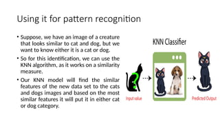
The k-nearest neighbor (k-NN) algorithm is a simple, non-parametric supervised learning technique used for classification and density estimation based on the similarity between data points. It is a lazy learner that does not learn from the training data until classification begins, and its performance depends significantly on the choice of k, the distance metric, and a balanced training set. The document also discusses applications in image recognition and the importance of distance measurement, highlighting the need for standardization of predictors and cross-validation to determine the most effective parameters.

1. CLASSIFICATION

2. Nearest Neighbor Learning

3. Basics
• K-Nearest Neighbour is one of the simplest Machine Learning algorithms
based on Supervised Learning technique.
• K-NN algorithm assumes the similarity between the new case/data and
available cases and put the new case into the category that is most similar
to the available categories.
• It is also called a lazy learner algorithm because it does not learn from the
training set immediately instead it stores the dataset and at the time of
classification, it performs an action on the dataset.
• K-NN is a non-parametric algorithm, which means it does not make any
assumption on underlying data.
• For any given problem, a small value of k will lead to a large variance in
predictions; Alternatively, setting k to a large value may lead to a large
model bias.

4. Using it for pattern recognition
• Suppose, we have an image of a creature
that looks similar to cat and dog, but we
want to know either it is a cat or dog.
• So for this identification, we can use the
KNN algorithm, as it works on a similarity
measure.
• Our KNN model will find the similar
features of the new data set to the cats
and dogs images and based on the most
similar features it will put it in either cat
or dog category.

5. Using it for pattern recognition
(Just one way to classify)

6. Using it for estimating the density functions
• There are several types of non-parametric methods of interest in
pattern recognition.
• It consists of procedures for estimating the density functions p(x|yq)
from sample patterns (without the assumption that forms of
underlying densities are known; and with the assumption that
attributes are statistically independent).
• In probability theory, a probability density function is a function
whose value at any given sample (or point) in the sample space (the
set of possible values) can be interpreted as providing a relative
likelihood that the value of the random variable would be close to
that sample.

7. Estimation of probability density function
• Assume that the sample {x(i)
}; i = 1,…, N, is drawn independently from
some unknown probability density p(.).
• (.) is our estimate of p(.).
• We start with the univariate case where x(i) are scalars (n = 1), and later
generalize to the multidimensional case.
• For the non-parametric estimation, the oldest and the most popular
method is the histogram, where the input space is divided into equal-
sized intervals, named bins.
• The corresponding probability is approximated by the frequency ratio:
where #{.} denotes the number of
training instances x(i)
that lie in the
same bin as the test instance x.

8. Estimation of probability density function
• This approximation converges to the true probability as N approaches infinity.
• The corresponding probability density function value is assumed constant
throughout the bin and is approximated as,
• where is the midpoint of the bin
• and h is the width of the bin.

9. Estimation of probability density function
• In constructing the histogram, we have to choose both an origin and a bin
width h.
• With small bins, the estimate is spiky, and with larger bins, the estimate is
smoother.
• There are discontinuities at the boundaries.
• For a large enough number of
samples, the smaller the h, the
better the accuracy of the resulting
estimate.
• Usually, a large N is necessary for
acceptable performance.

10. Estimation of probability density function
• The nearest-neighbor class of estimators adopts the reasonable amount of
smoothing to the local density of the data.
• The degree of smoothing is controlled by k (the number of neighbors taken
into account), which is much smaller than N (the sample size).
• For each x (n = 1), we define distances from x
to the points in the sample.
• The k-nearest neighbor (k-NN) density estimate is
• instead of fixing h and checking how many samples fall in the bin, we fix k,
the number of observations to fall in the bin, and compute the bin size.
• Where density is high, bins are small, and where density is low, bins are
larger.

11. Estimation of probability density function
• Generalizing to multivariable data,
• where Vk(x) is the volume of the n-dimensional hyperspace centered at x
with radius r = ||x – x(k)||; x(k) is the kth
nearest observation to x among the
neighbors.
• When used for classification, we need the class-conditional densities, p(x|yq)
of the feature vector distributions.
• The estimator of the class-conditional density is given as,
• where kq is the number of neighbors out of k nearest that belong to class yq;
and Nq is the number of labeled instances belonging to class yq.

12. Estimating a posteriori probabilities using KNN
Thus, the estimate of the a posteriori
probability that yq is the class for sample x is
just the fraction of the samples within the
cell Vk(x) that are labeled yq.
(yq is the class for sample x)

13. KNN Classification

14. Computer Vision: Car detection
Testing:
What is this?
Not a car
Cars

15. (Histogram of Oriented Gradients)

16. You see this:
But the camera sees this:
What is this?

17. Learning
Algorithm
pixel 1
pixel 2
pixel 1
pixel 2
Raw image
Cars
“Non”-Cars

18. (Local Binary Pattern)
To find the image that
matches the input image
we just need to compare
two histograms and
return the image with
the closest histogram
(based on distance).

19. How does it work?
• We first determine the k points that are closest neighbors of x with the help
of a specific distance metric.
• The categorization of x is then given by the class label found in most of the k
neighbors.
• All neighbors have equal vote, and the class with the most number of votes
among the k neighbors is selected.
• Ties are randomly broken or weighted vote is taken.
• k is usually taken an odd number to reduce ties: confusion exists usually
between two neighboring classes.
• Note that k = 1 is usually not sufficient for determining the class of x due to
noise and outliers in the data.
• A set of nearest neighbors is needed to accurately decide the class.

20. Distance function?
• The key issue of k-NN algorithm is the distance/similarity function, which is
selected on the basis of applications and nature of the data.
• The cautious selection of an appropriate distance function is a crucial step in
the use of k-NN.
• A validation set can be made use of to pick the appropriate distance
function for a given dataset by applying all candidates to gauge which one
gives better results.

21. Value of k?
• Another question is the number of neighbors to select.
• Again, investigation of varying numbers of neighbors with the help of the
validation set can facilitate establishing the optimal number, as the number
is dependent on the data distribution and relies heavily on the problem
being solved.
• Selecting the appropriate training set is probably the most important step in
k-NN process.
• The training set should include enough examples of all probable categories,
that is, it should be a balanced training set having more or less the same
number of instances for all classes.
• Generally speaking, the size of the training set should have at least
thousands, if not hundreds of thousands or millions, of training examples.

22. Value of k?
• The data is partitioned into training, validation, and test sets.
• Validation set is used to compare error rates for various values of k/various
similarity measures, and test set is used to evaluate the performance.
• In the k-NN procedure, all neighbors have equal vote.
• In an alternative method: the Parzon-window approach, also called
Probabilistic Neural Network (PNN), the weight of the vote is given by a
kernel function, typically giving more weight to closer instances.
• Low k-value is sensitive to outliers and a higher K-value is more resilient to
outliers as it considers more voters to decide prediction.

23. Value of k?
• Cross-validation is a smart way to find out the optimal K value.
• It estimates the validation error rate by holding out a subset of the training set
from the model building process.
• Cross-validation (let's say 10 fold validation) involves randomly dividing the
training set into 10 groups, or folds, of approximately equal size.
• 90% data is used to train the model and remaining 10% to validate it.
• The misclassification rate is then computed on the 10% validation data.
• This procedure repeats 10 times.
• Different group of observations are treated as a validation set each of the 10
times.
• It results to 10 estimates of the validation error which are then averaged out.

24. Pros and Cons of KNN
Pros Cons
Easy to understand Memory Intensive / Computationally
expensive
No assumptions about data Sensitive to scale of data
Can be applied to both classification and
regression
Not work well on rare event (skewed)
target variable
Works easily on multi-class problems Struggle when high number of
independent variables

25. Numerical Discussion

26. Example 1:
• Consider the following data concerning credit default. Age and Loan
are two numerical variables (predictors) and Default is the target.

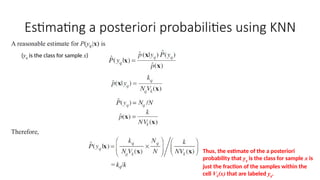
27. Example 1:
• We can now use the training set to
classify an unknown case (Age=48 and
Loan=$142,000) using Euclidean
distance.
• If K=1 then the nearest neighbor is the
last case in the training set with
Default=Y.
• D = Sqrt[(48-33)^2 + (142000-
150000)^2] = 8000.01 >> Default=Y
• With K=3, there are two “Default=Y”
and one “Default=N” out of three
closest neighbors. The prediction for
the unknown case is again Default=Y.

28. Example 1:
• One major drawback in calculating
distance measures directly from the
training set is in the case where variables
have different measurement scales or
there is a mixture of numerical and
categorical variables.
• For example, if one variable is based on
annual income in dollars, and the other is
based on age in years then income will
have a much higher influence on the
distance calculated.
• One solution is to standardize the training
set as shown here.
Using the standardized distance on the same training
set, the unknown case returned a different neighbor
which is not a good sign of robustness.
Standardized Distance

29. Example 2:
• Suppose we have height, weight and T-shirt size of some
customers and we need to predict the T-shirt size of a
new customer given only height and weight information
we have.
• Data including height, weight and T-shirt size information
is shown here
• Step 1 : Calculate Similarity based on distance function
• There are many distance functions but Euclidean is the
most commonly used measure.
• It is mainly used when data is continuous. Manhattan
distance is also very common for continuous variables.

30. Example 2:
• The idea to use distance measure is to find the distance (similarity) between
new sample and training cases and then finds the k-closest customers to
new customer in terms of height and weight.
• New customer named 'Monica' has height 161cm and weight 61kg.
• Euclidean distance between first observation and new observation (monica)
is as follows - d=SQRT((161-158)^2+(61-58)^2)
• Similarly, we will calculate distance of all the
training cases with new case and calculates
the rank in terms of distance.
• The smallest distance value will be ranked 1
and considered as nearest neighbor.

31. Example 2:
• Step 2 : Find K-Nearest Neighbors
• Let k be 5.
• Then the algorithm searches for the 5
customers closest to Monica, i.e. most
similar to Monica in terms of attributes,
and see what categories those 5
customers were in.
• If 4 of them had ‘Medium T shirt sizes’
and 1 had ‘Large T shirt size’ then your
best guess for Monica is ‘Medium T shirt.
• See the calculation shown in the figure.

32. Example 2:
• In the graph, binary dependent variable
(T-shirt size) is displayed in blue and
orange color.
• 'Medium T-shirt size' is in blue color
and 'Large T-shirt size' in orange color.
• New customer information is exhibited
in yellow circle.
• Four blue highlighted data points and
one orange highlighted data point are
close to yellow circle.
• So the prediction for the new case is
blue highlighted data point which is
Medium T-shirt size.

33. Example 2:
• Standardization
• In order to make the values comparable we need to
standardize them which can be done by any of the
following methods :
• After standardization, 5th closest value got changed as
height was dominating earlier before standardization.
Hence, it is important to standardize predictors before
running K-nearest neighbor algorithm.

34. Assessing Classification Accuracy
Misclassification Error
• Metric for assessing the accuracy of classification algorithms is:
number of samples misclassified by the model
• For binary classification problems,
• For 0% error, for all data points