Downloaded 734 times
![K-means clustering
N
∑ K
∑
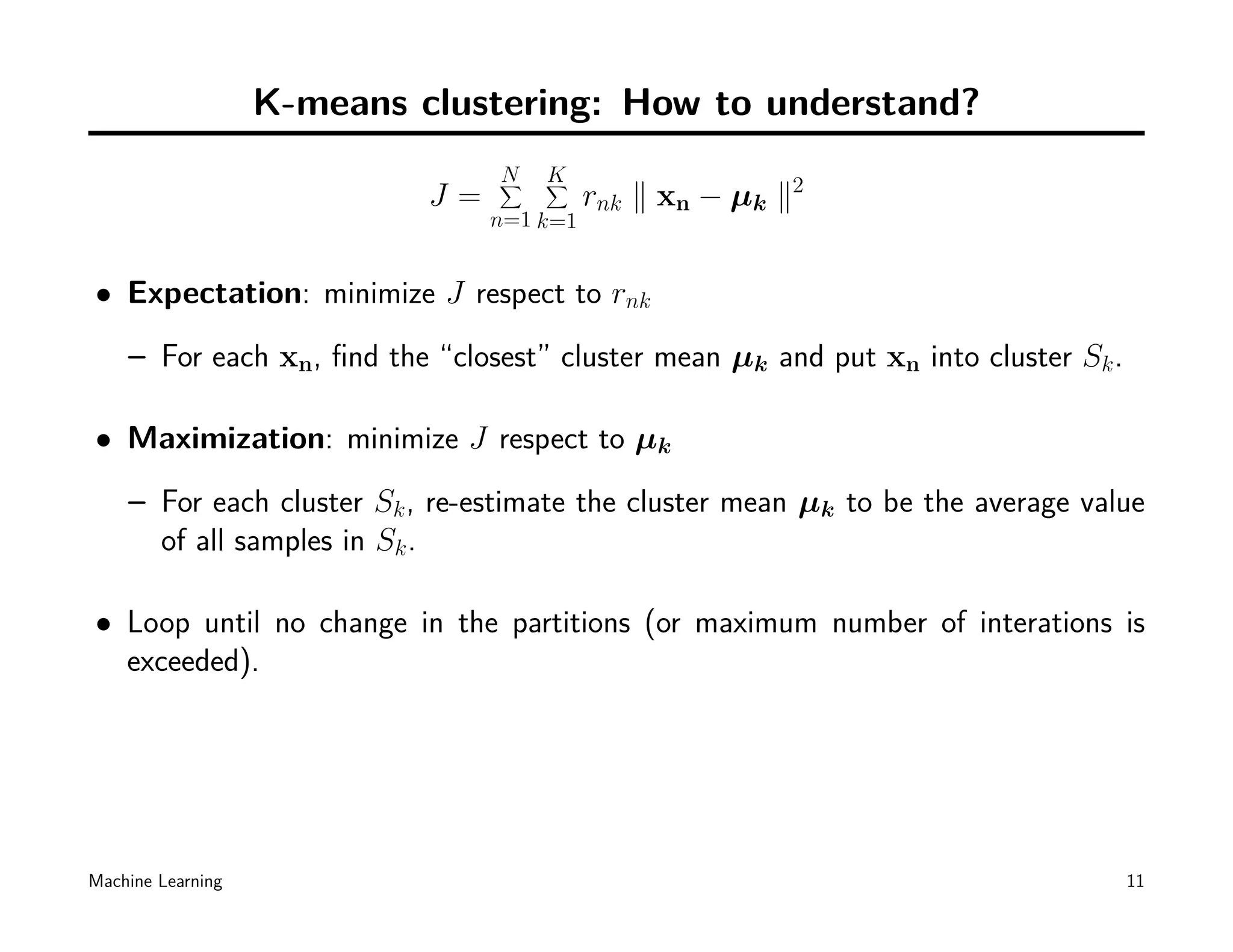
J= rnk ∥ xn − µk ∥2
n=1 k=1
• Expectation: J is linear function of rnk
1 if k = arg minj ∥ xn − µj ∥2
rnk =
0
otherwise
• Maximization: setting the derivative of J with respect to µk to zero, gives:
∑
n rnk xn
µk = ∑
n rnk
Convergence of K-means: assured [why?], but may lead to local minimum of J
[8]
Machine Learning 10](https://image.slidesharecdn.com/gmm-101010112502-phpapp01/75/K-means-EM-and-Mixture-models-11-2048.jpg)
![K-means clustering: some variations
• Initial cluster centroids:
– Randomly selected
– Iterative procedure: k-mean++ [2]
• Number of clusters K:
√
– Empirically/experimentally: 2 ∼ n
– Learning [6]
• Objective function:
– General dissimilarity measure: k-medoids algorithm.
• Speeding up:
– kd-trees for pre-processing [7]
– Triangle inequality for distance calculation [4]
Machine Learning 13](https://image.slidesharecdn.com/gmm-101010112502-phpapp01/75/K-means-EM-and-Mixture-models-14-2048.jpg)
![Expectation Maximization
• A general-purpose algorithm for MLE in a wide range of situations.
• First formally stated by Dempster, Laird and Rubin in 1977 [1]
– We even have several books discussing only on EM and its variations!
• An excellent way of doing our unsupervised learning problem, as we will see
– EM is also used widely in other domains.
Machine Learning 16](https://image.slidesharecdn.com/gmm-101010112502-phpapp01/75/K-means-EM-and-Mixture-models-17-2048.jpg)
![EM: a solution for MLE
• Given a statistical model with:
– a set X of observed data,
– a set Z of unobserved latent data,
– a vector of unknown parameters θ,
– a likelihood function L (θ; X, Z) = p (X, Z | θ)
• Roughly speaking, the aim of MLE is to determine θ = arg maxθ L (θ; X, Z)
– We known the old trick: partial derivatives of the log likelihood...
– But it is not always tractable [e.g.]
– Other solutions are available.
Machine Learning 17](https://image.slidesharecdn.com/gmm-101010112502-phpapp01/75/K-means-EM-and-Mixture-models-18-2048.jpg)
![EM: General Case
L (θ; X, Z) = p (X, Z | θ)
• EM is just an iterative procedure for finding the MLE
• Expectation step: keep the current estimate θ (t) fixed, calculate the expected
value of the log likelihood function
( )
Q θ|θ (t)
= E [log L (θ; X, Z)] = E [log p (X, Z | θ)]
• Maximization step: Find the parameter that maximizes this quantity
( )
θ (t+1)
= arg max Q θ | θ (t)
θ
Machine Learning 18](https://image.slidesharecdn.com/gmm-101010112502-phpapp01/75/K-means-EM-and-Mixture-models-19-2048.jpg)
![EM Convergence
• E.M. Convergence: Yes
– After each iteration, p (X, Z | θ) must increase or remain [NOT OBVIOUS]
– But it can not exceed 1 [OBVIOUS]
– Hence it must converge [OBVIOUS]
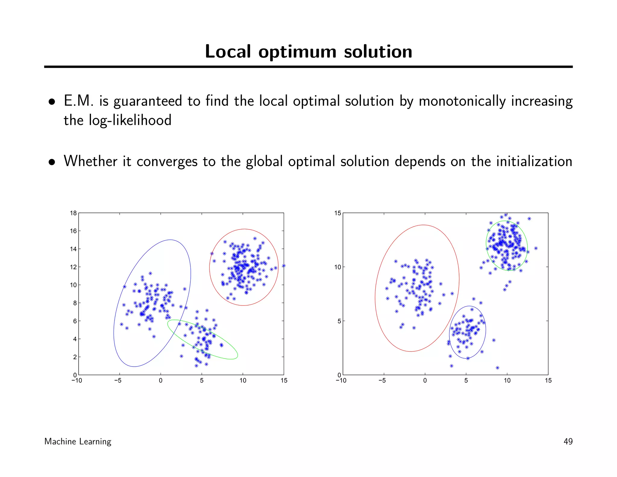
• Bad news: E.M. converges to local optimum.
– Whether the algorithm converges to the global optimum depends on the ini-
tialization.
• Let’s take K-means as an example, again...
• Details can be found in [9].
Machine Learning 21](https://image.slidesharecdn.com/gmm-101010112502-phpapp01/75/K-means-EM-and-Mixture-models-22-2048.jpg)
![Regularized EM (REM)
• EM tries to inference the latent (missing) data Z from the observations X
– We want to choose the missing data that has a strong probabilistic relation
to the observations, i.e. we assume that the observations contains lots of
information about the missing data.
– But E.M. does not have any control on the relationship between the missing
data and the observations!
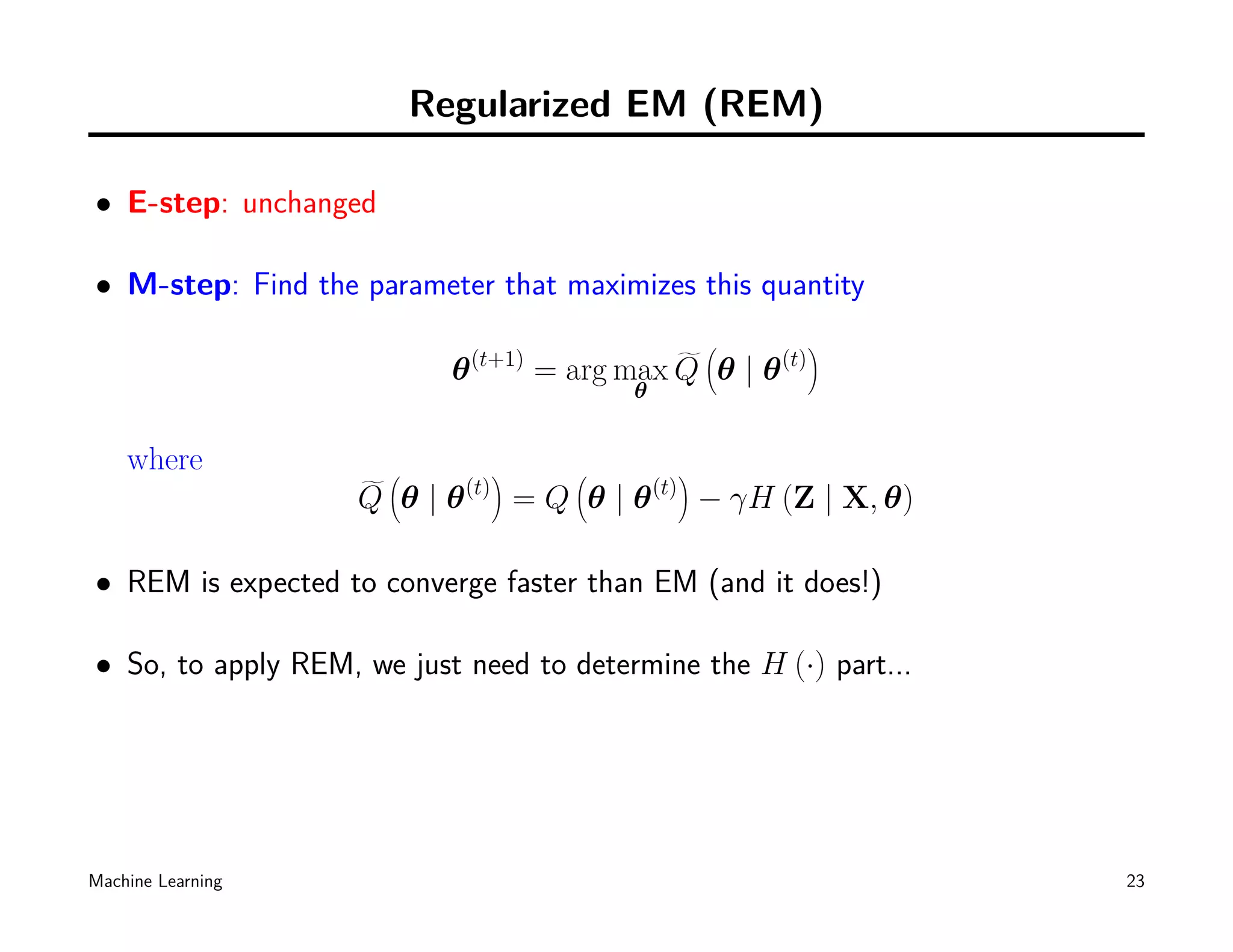
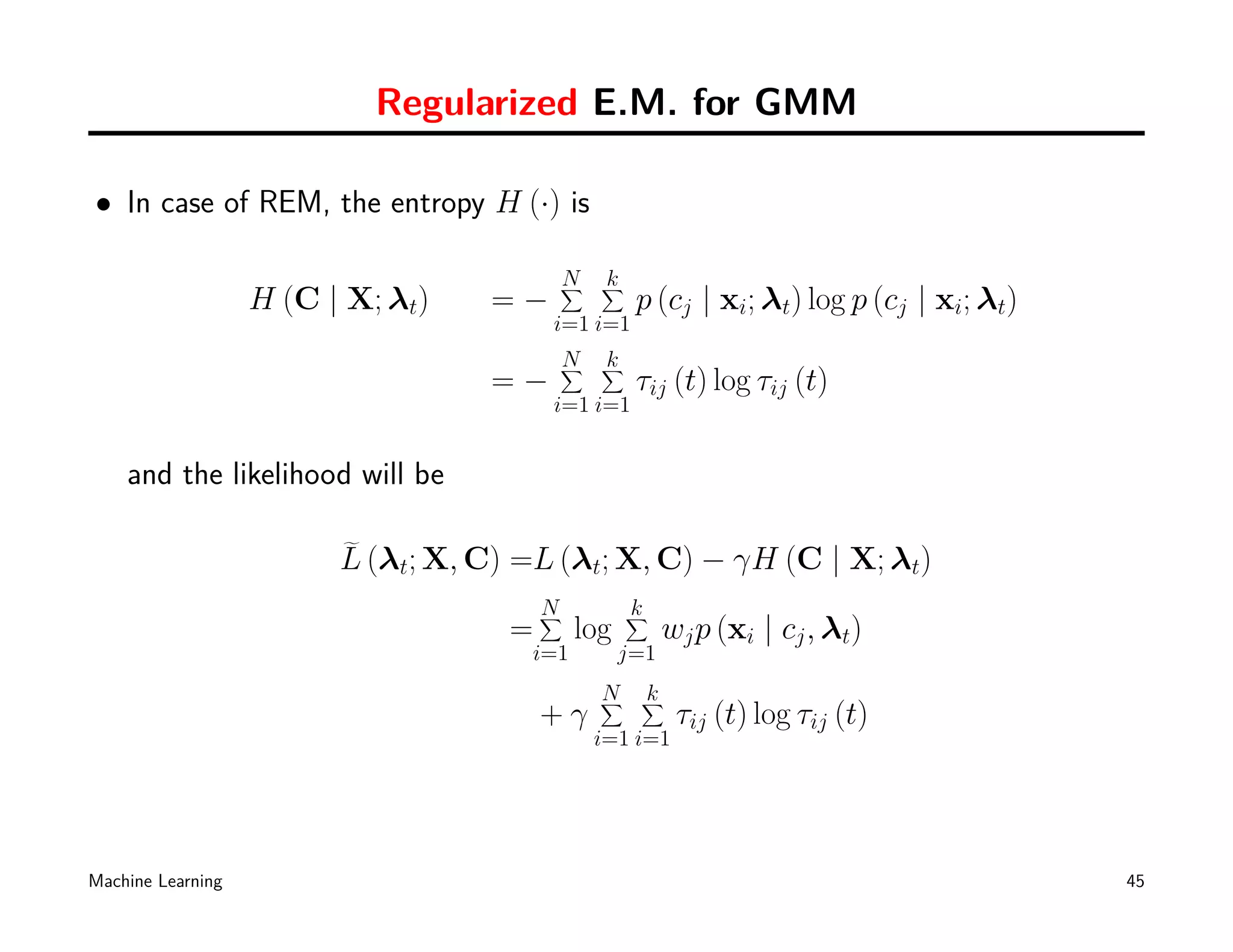
• Regularized EM (REM) [5] tries to optimized the penalized likelihood
L (θ | X, Z) = L (θ | X, Z) − γH (Z | X, θ)
where H (Y ) is Shannon’s entropy of the random variable Y :
∑
H (Y ) = − p (y) log p (y)
y
and the positive value γ is the regularization parameter. [When γ = 0?]
Machine Learning 22](https://image.slidesharecdn.com/gmm-101010112502-phpapp01/75/K-means-EM-and-Mixture-models-23-2048.jpg)
![Remind: Bayes Classifier
70
60
50
40
30
20
10
0
−10
0 10 20 30 40 50 60 70 80
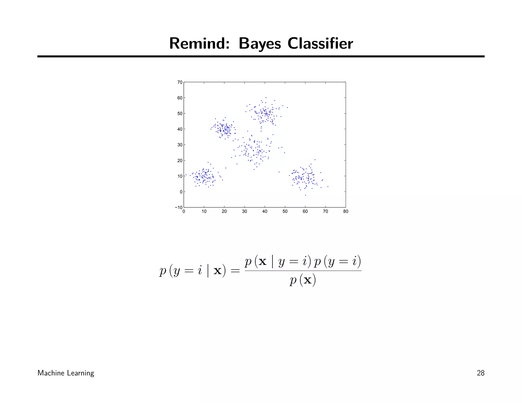
In case of Gaussian Bayes Classifier:
[ ]
T
d/2
1
exp −2
1
(x − µi) Σi (x − µi) pi
(2π) ∥Σi ∥1/2
p (y = i | x) =
p (x)
How can we deal with the denominator p (x)?
Machine Learning 29](https://image.slidesharecdn.com/gmm-101010112502-phpapp01/75/K-means-EM-and-Mixture-models-30-2048.jpg)
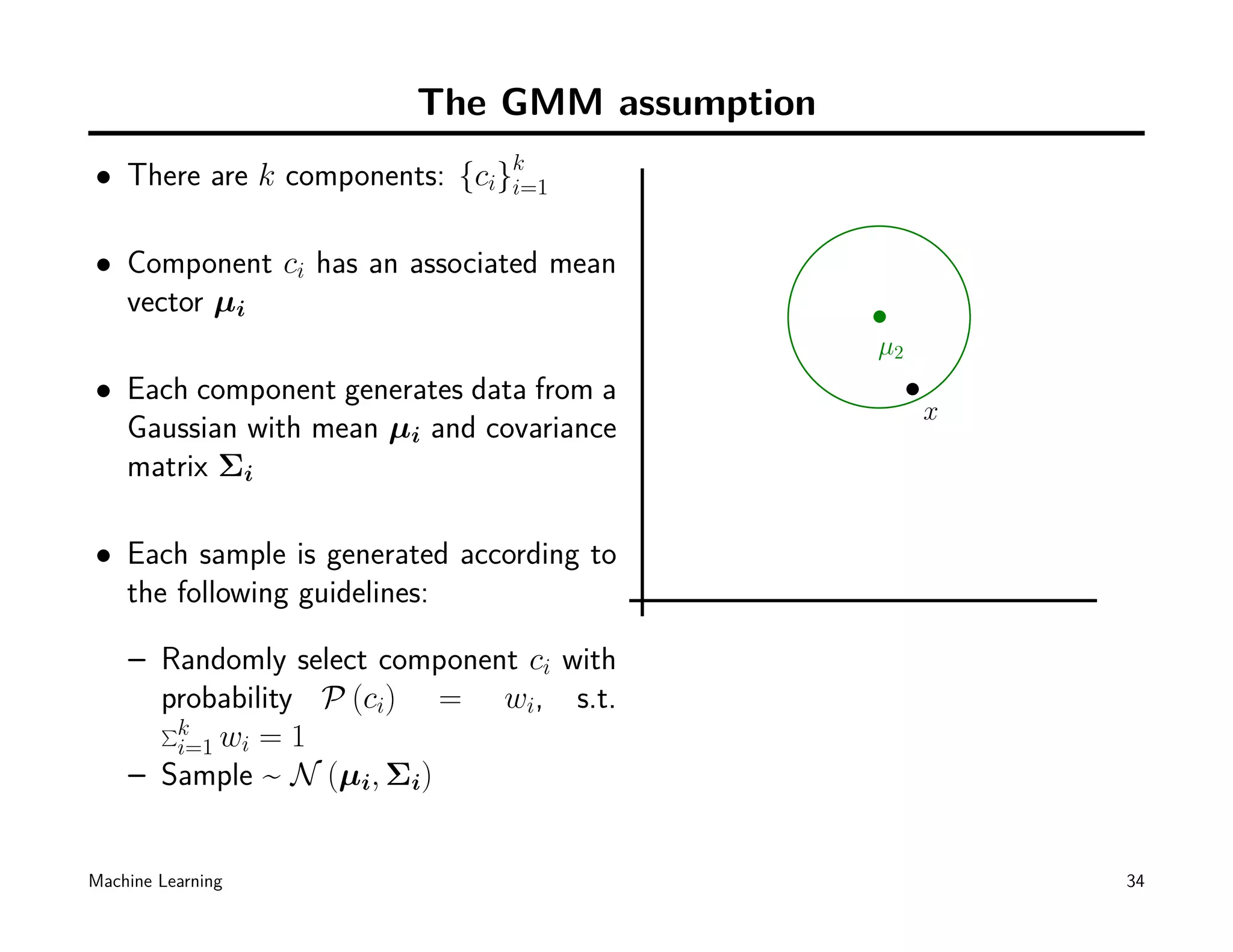
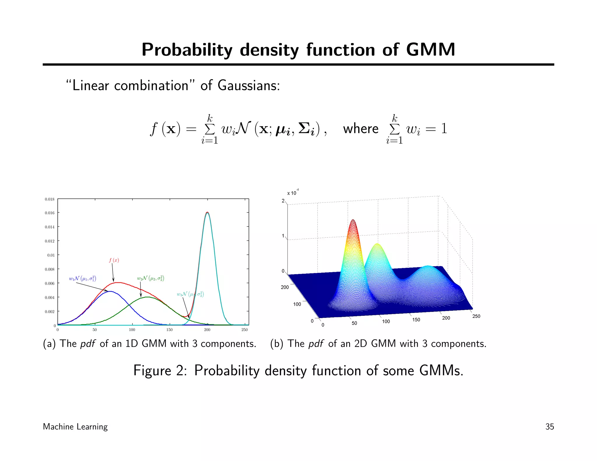

![Computing likelihoods in unsupervised case
k
∑ k
∑
f (x) = wiN (x; µi, Σi) , where wi = 1
i=1 i=1
• Given a mixture of Gaussians, denoted by G. For any x, we can define the
likelihood:
P (x | G) = P (x | w1, µ1, Σ1, ..., wk , µk , Σk )
k
∑
= P (x | ci) P (ci)
i=1
k
∑
= wiN (x; µi, Σi)
i=1
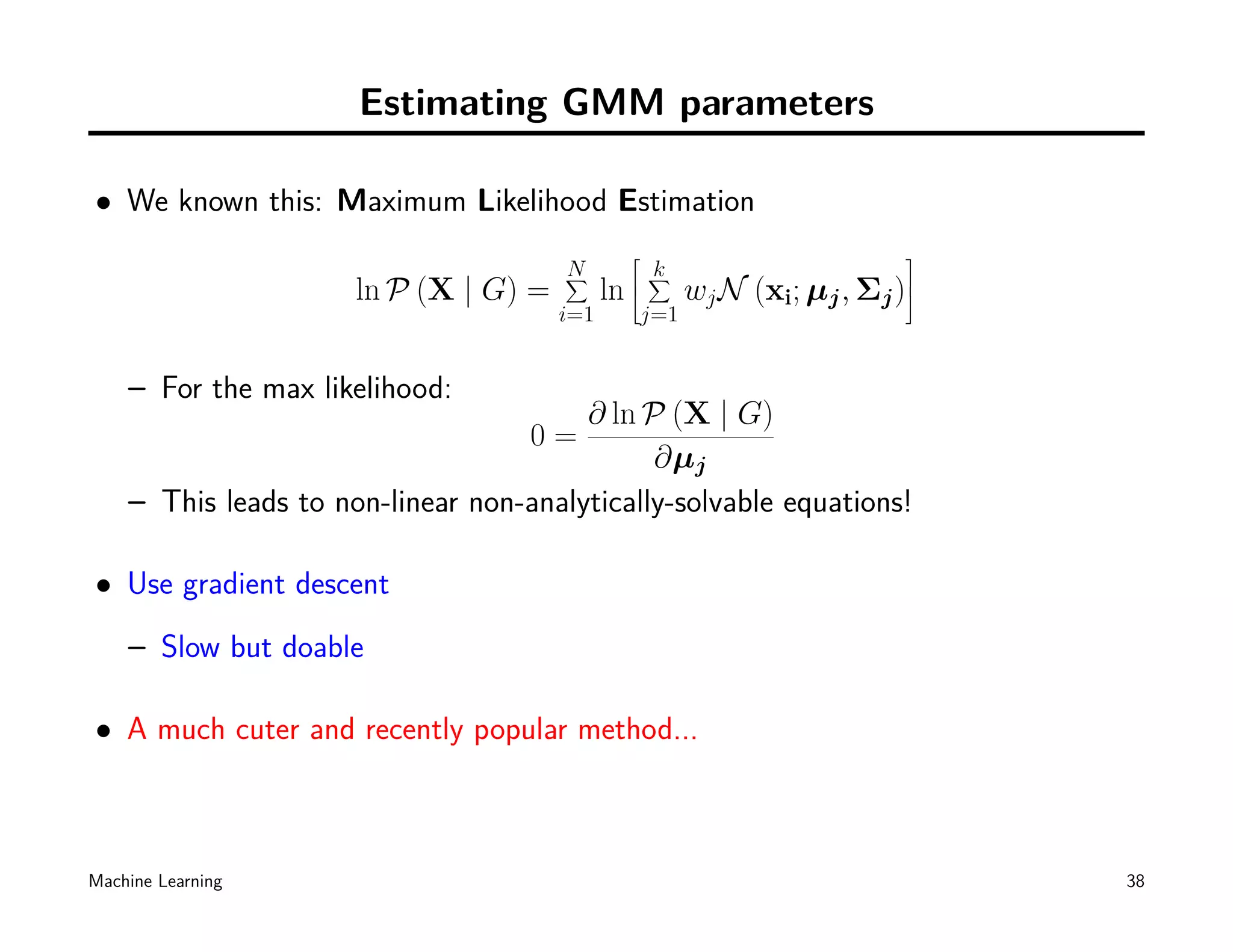
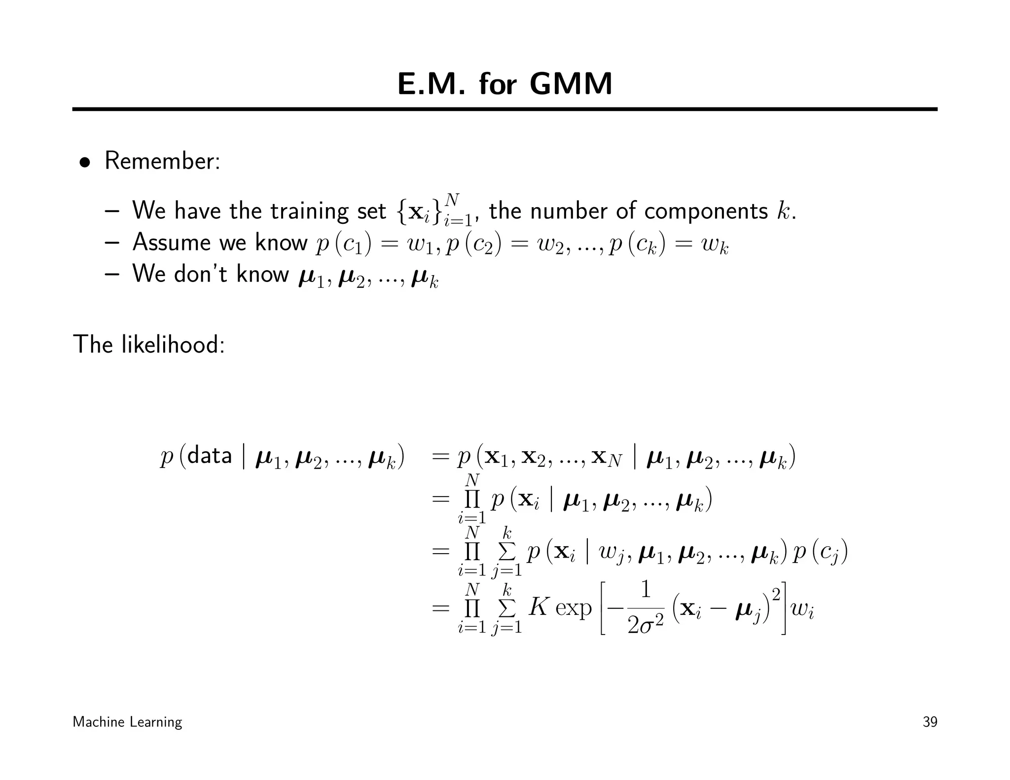
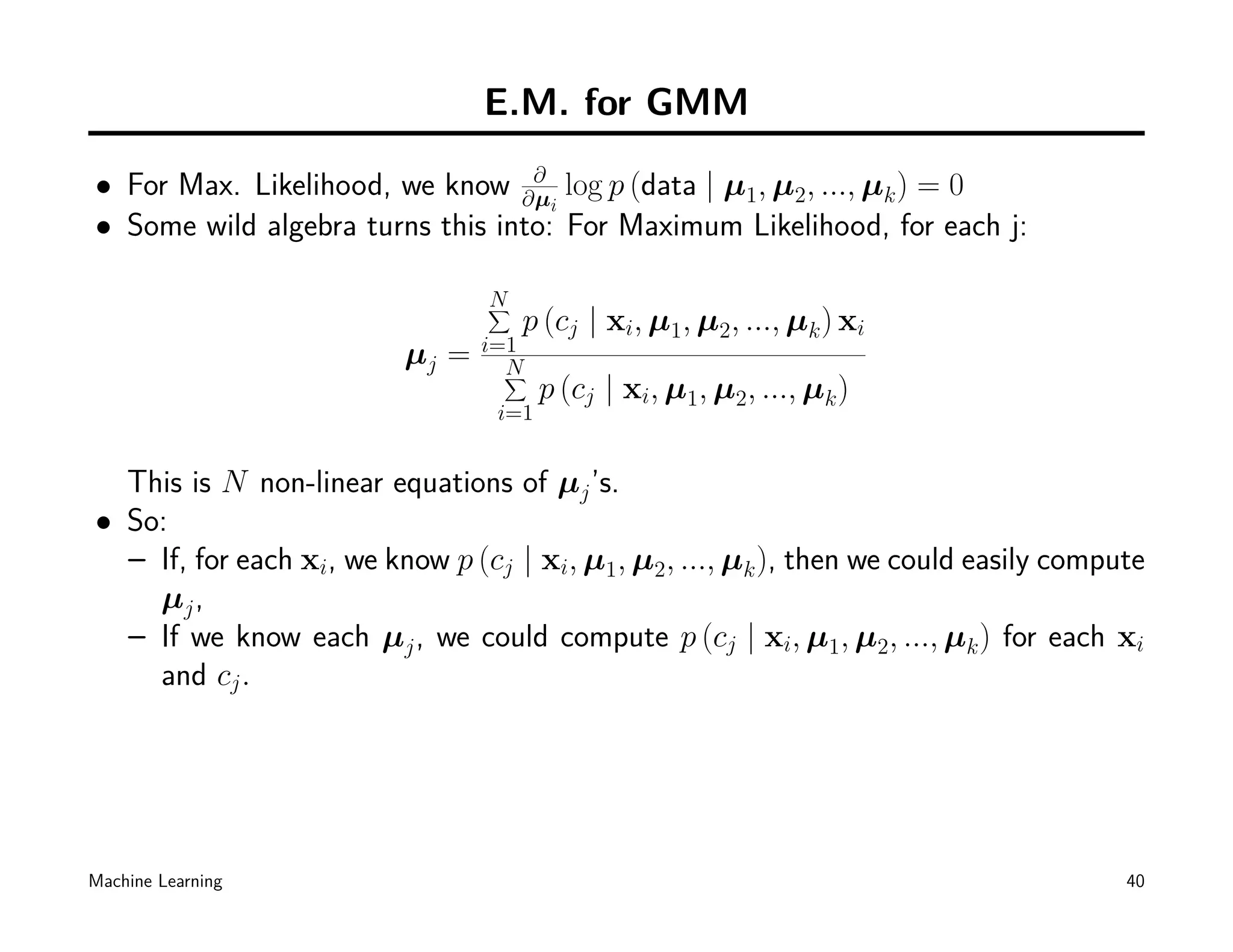
• So we can define likelihood for the whole training set [Why?]
N
∏
P (x1, x2, ..., xN | G) = P (xi | G)
i=1
N ∑
∏ k
= wj N (xi; µj , Σj )
i=1 j=1
Machine Learning 37](https://image.slidesharecdn.com/gmm-101010112502-phpapp01/75/K-means-EM-and-Mixture-models-38-2048.jpg)
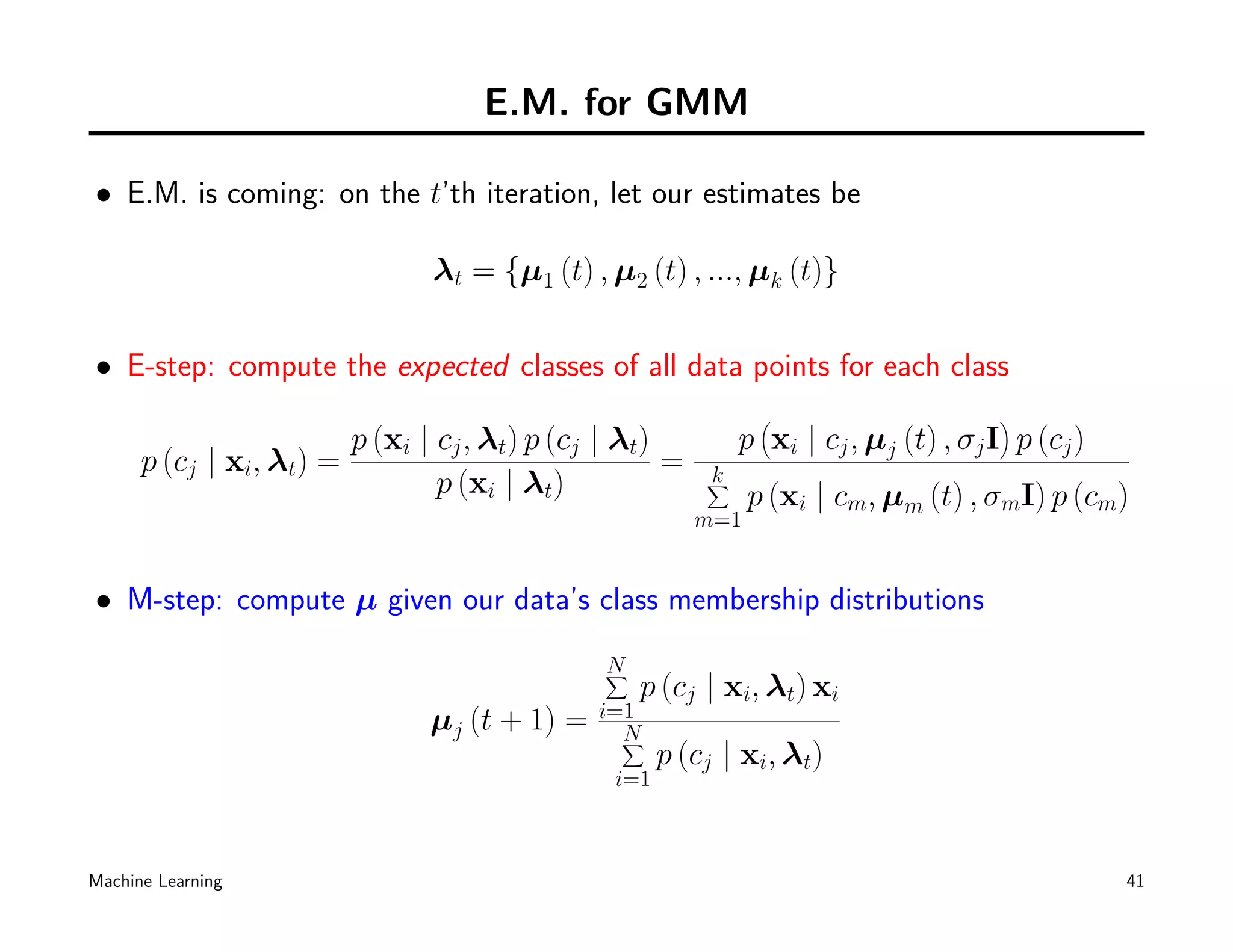
![E.M. for General GMM: M-step
• M-step: compute µ given our data’s class membership distributions
N
∑ N
∑
p (cj | xi, λt) p (cj | xi, λt) xi
i=1 i=1
wj (t + 1) = µj (t + 1) = N
N ∑
p (cj | xi, λt)
i=1
1 N
∑ 1 N
∑
= τij (t) = τij (t) xi
N i=1 N wj (t + 1) i=1
N
∑ [ ][ ]
T
p (cj | xi, λt) xi − µj (t + 1) xi − µj (t + 1)
i=1
Σj (t + 1) = N
∑
p (cj | xi, λt)
i=1
1 N
∑ [ ][ ]
T
= τij (t) xi − µj (t + 1) xi − µj (t + 1)
N wj (t + 1) i=1
Machine Learning 43](https://image.slidesharecdn.com/gmm-101010112502-phpapp01/75/K-means-EM-and-Mixture-models-44-2048.jpg)

![Regularized E.M. for GMM
• Some algebra [5] turns into:
N
∑
p (cj | xi, λt) (1 + γ log p (cj | xi, λt))
i=1
wj (t + 1) =
N
1 N
∑
= τij (t) (1 + γ log τij (t))
N i=1
N
∑
p (cj | xi, λt) xi (1 + γ log p (cj | xi, λt))
µj (t + 1) = i=1
N
∑
p (cj | xi, λt) (1 + γ log p (cj | xi, λt))
i=1
1 N
∑
= τij (t) xi (1 + γ log τij (t))
N wj (t + 1) i=1
Machine Learning 46](https://image.slidesharecdn.com/gmm-101010112502-phpapp01/75/K-means-EM-and-Mixture-models-47-2048.jpg)
![Regularized E.M. for GMM
• Some algebra [5] turns into (cont.):
1 N
∑
Σj (t + 1) = τij (t) (1 + γ log τij (t)) dij (t + 1)
N wj (t + 1) i=1
where [ ][ ]
T
dij (t + 1) = xi − µj (t + 1) xi − µj (t + 1)
Machine Learning 47](https://image.slidesharecdn.com/gmm-101010112502-phpapp01/75/K-means-EM-and-Mixture-models-48-2048.jpg)
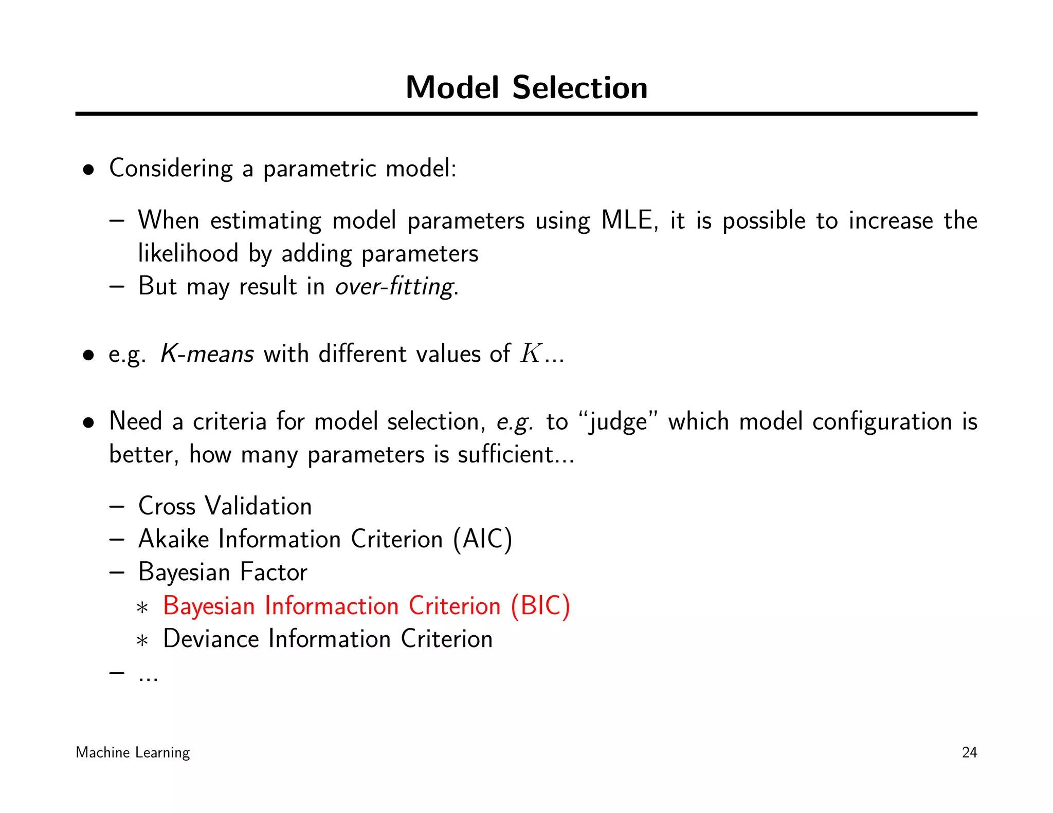
![GMM: Model Selection
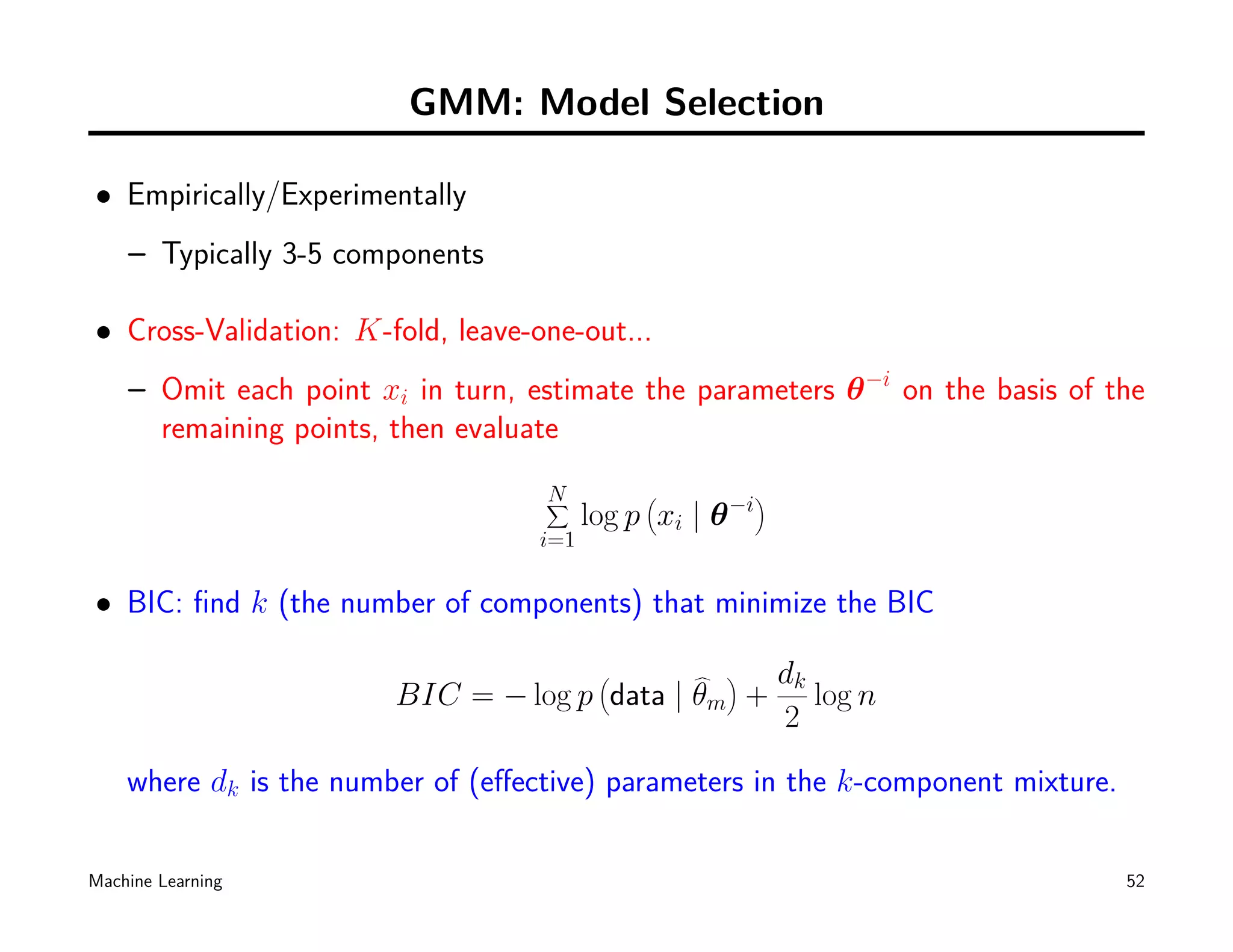
• Empirically/Experimentally [Sure!]
• Cross-Validation [How?]
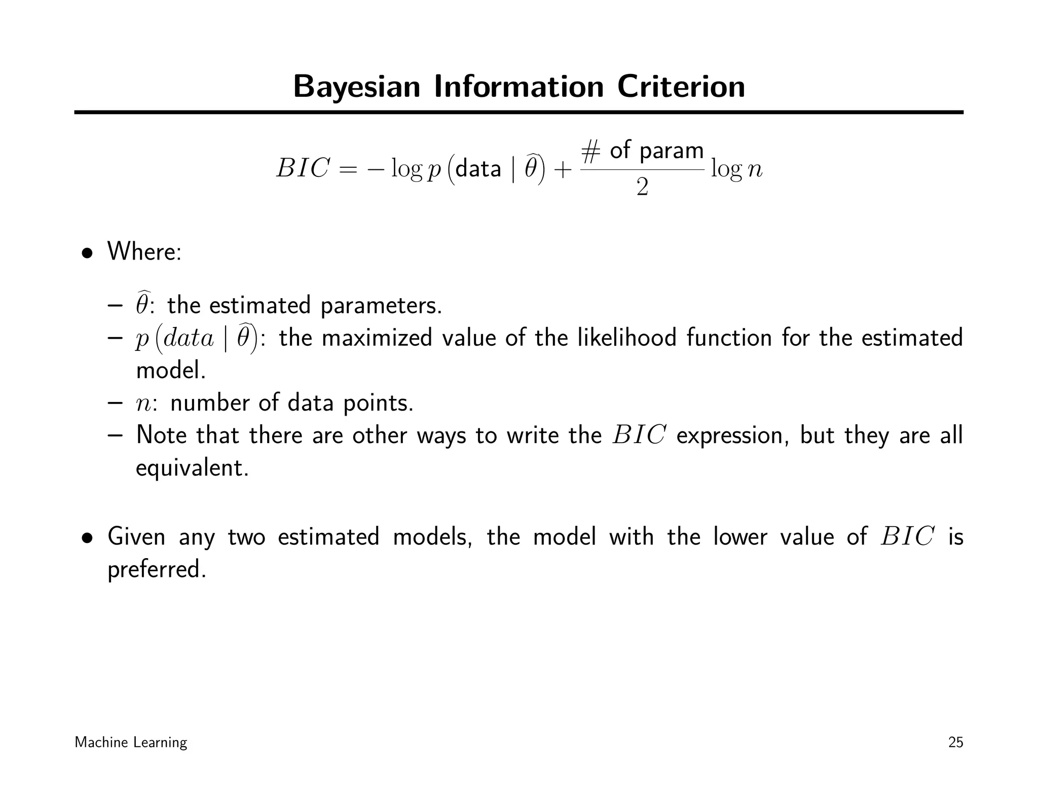
• BIC
• ...
Machine Learning 51](https://image.slidesharecdn.com/gmm-101010112502-phpapp01/75/K-means-EM-and-Mixture-models-52-2048.jpg)
![What you should already know?
• K-means as a trivial classifier
• E.M. - an algorithm for solving many MLE problems
• GMM - a tool for modeling data
– Note 1: We can have a mixture model of many different types of distribution,
not only Gaussians
– Note 2: Compute the sum of Gaussians may be expensive, some approximations
are available [3]
• Model selection:
– Bayesian Information Criterion
Machine Learning 58](https://image.slidesharecdn.com/gmm-101010112502-phpapp01/75/K-means-EM-and-Mixture-models-59-2048.jpg)
![References
[1] N. Laird A. Dempster and D. Rubin. Maximum likelihood from incomplete data
via the em algorithm. Journal of the Royal Statistical Society. Series B (Method-
ological), 39(1):pp. 1–38., 1977.
[2] David Arthur and Sergei Vassilvitskii. k-means ++ : The Advantages of Careful
Seeding. In Proceedings of the eighteenth annual ACM-SIAM symposium on
Discrete algorithms, volume 8, pages 1027–1035, 2007.
[3] N. Gumerov C. Yang, R. Duraiswami and L. Davis. Improved fast gauss transform
and efficient kernel density estimation. In IEEE International Conference on
Computer Vision, pages pages 464–471, 2003.
[4] Charles Elkan. Using the Triangle Inequality to Accelerate k-Means. In Proceed-
Machine Learning 60](https://image.slidesharecdn.com/gmm-101010112502-phpapp01/75/K-means-EM-and-Mixture-models-61-2048.jpg)
![ings of the Twentieth International Conference on Machine Learning (ICML),
2003.
[5] Keshu Zhang Haifeng Li and Tao Jiang. The regularized em algorithm. In
Proceedings of the 20th National Conference on Artificial Intelligence, pages
pages 807 – 812, Pittsburgh, PA, 2005.
[6] Greg Hamerly and Charles Elkan. Learning the k in k-means. In In Neural
Information Processing Systems. MIT Press, 2003.
[7] Tapas Kanungo, David M Mount, Nathan S Netanyahu, Christine D Piatko, Ruth
Silverman, and Angela Y Wu. An efficient k-means clustering algorithm: anal-
ysis and implementation. IEEE Transactions on Pattern Analysis and Machine
Intelligence, 24(7):881–892, July 2002.
[8] J MacQueen. Some methods for classification and analysis of multivariate obser-
vations. In Proceedings of 5th Berkeley Symposium on Mathematical Statistics
and Probability, volume 233, pages 281–297. University of California Press, 1967.
Machine Learning 61](https://image.slidesharecdn.com/gmm-101010112502-phpapp01/75/K-means-EM-and-Mixture-models-62-2048.jpg)
![[9] C.F. Wu. On the convergence properties of the em algorithm. The Annals of
Statistics, 11:95–103, 1983.
Machine Learning 62](https://image.slidesharecdn.com/gmm-101010112502-phpapp01/75/K-means-EM-and-Mixture-models-63-2048.jpg)

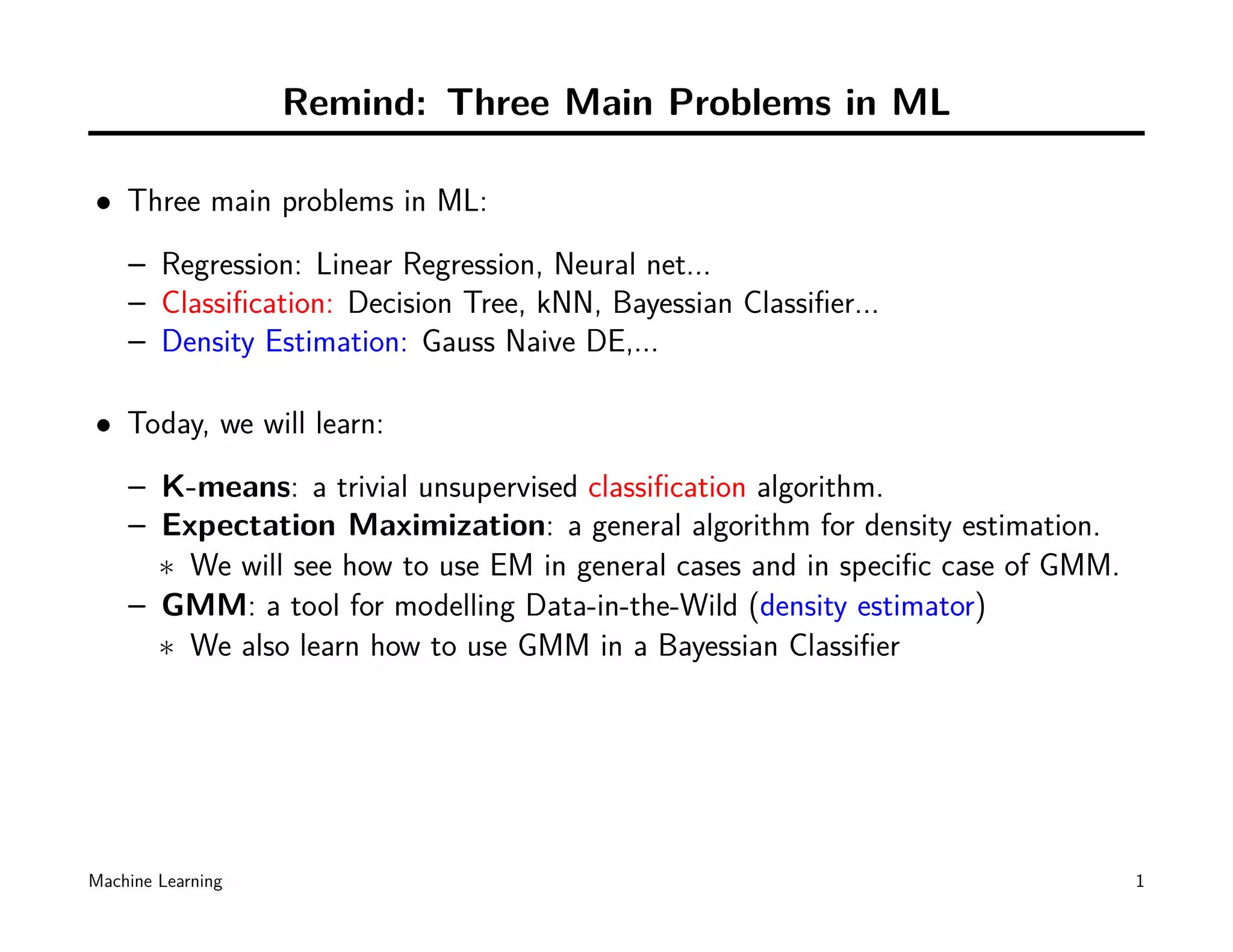
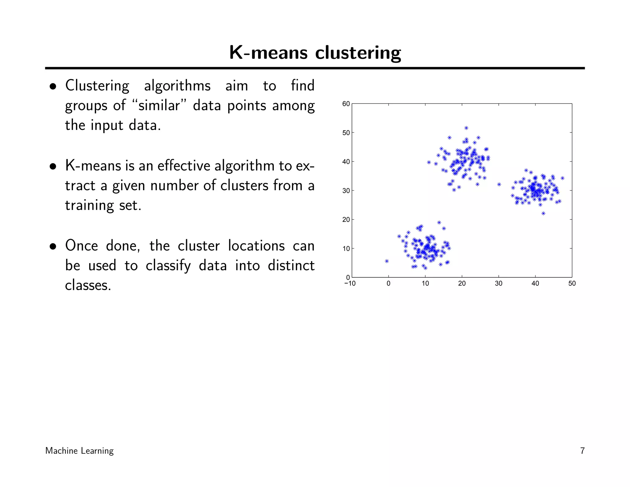
This document discusses machine learning techniques including k-means clustering, expectation maximization (EM), and Gaussian mixture models (GMM). It begins by introducing unsupervised learning problems and k-means clustering. It then describes EM as a general algorithm for maximum likelihood estimation and density estimation. Finally, it discusses using GMM with EM to model data distributions and for classification tasks.


![[PRML勉強会資料] パターン認識と機械学習 第3章 線形回帰モデル (章頭-3.1.5)(p.135-145)](https://cdn.slidesharecdn.com/ss_thumbnails/prmlp-150228215621-conversion-gate01-thumbnail.jpg?width=640&height=640&fit=bounds)