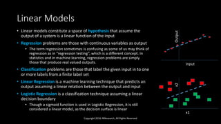
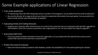
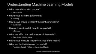
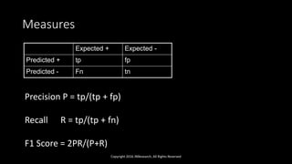
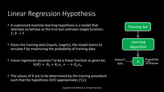
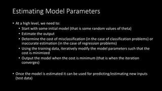
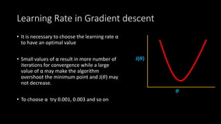
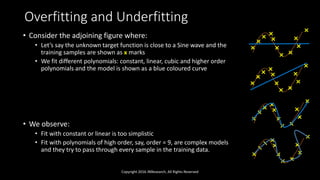
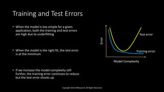
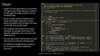
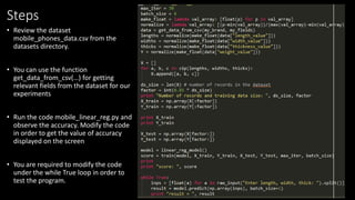
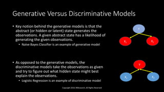
The document discusses linear models in machine learning, specifically focusing on linear and logistic regression techniques, their applications, and frameworks for training and evaluating models. It details concepts such as overfitting, underfitting, regularization, and optimization methods like gradient descent, while also addressing classification problems. Additionally, it introduces multiclass classification methods and the softmax classifier, offering insights into their operational mechanics and real-world applications.


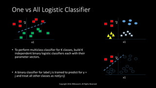

![[PR12] You Only Look Once (YOLO): Unified Real-Time Object Detection](https://cdn.slidesharecdn.com/ss_thumbnails/yolo-170616085751-thumbnail.jpg?width=640&height=640&fit=bounds)