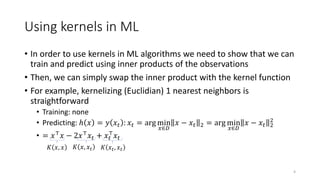
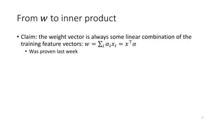
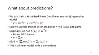
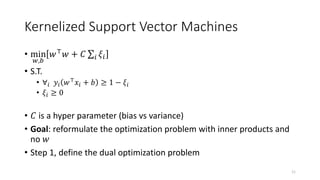
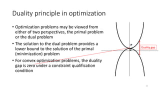
This document summarizes a machine learning course on kernel machines. The course covers feature maps that transform data into higher dimensional spaces to allow nonlinear models to fit complex patterns. It discusses how kernel functions can efficiently compute inner products in these transformed spaces without explicitly computing the feature maps. Specifically, it shows how support vector machines, linear regression, and other algorithms can be kernelized by reformulating them to optimize based on inner products between examples rather than model weights.

1. CSCE-421 Machine Learning
13. Kernel Machines
Instructor: Guni Sharon, classes: TR 3:55-5:10, HRBB 124
Based on a lecture by Kilian Weinberger and Joaquin Vanschoren 0

2. Announcements
• Midterm on Tuesday, November-23 (in class)
• Due:
• Quiz 4: ML debugging and kernelization, due Nov 4
• Assignment (P3): SVM, linear regression and kernelization, due Tuesday Nov-
16
1

3. Feature Maps
• Linear models: 𝑦 = 𝑤⊤𝑥 = 𝑖 𝑤𝑖𝑥𝑖 = 𝑤1𝑥1 + ⋯ + 𝑤𝑝𝑥𝑝
• When we cannot fit the data well (non-linear), add non-linear
combinations of features
• Feature map (or basis expansion ) 𝜙 ∶ 𝑋 → ℝ𝑑
𝑦 = 𝑤⊤𝑥 → 𝑦 = 𝑤⊤𝜙(𝑥)
• E.g., Polynomial feature map: all polynomials up to degree 𝑑
𝜙[1, 𝑥1, … , 𝑥𝑝] → [1, 𝑥1, … , 𝑥𝑝, 𝑥1
2
, … , 𝑥𝑝
2, … , 𝑥𝑝
𝑑, 𝑥1𝑥2, … , 𝑥𝑖𝑥𝑗]
• Example with p=1,d=3
𝑦 = 𝑤1𝑥1 → 𝑦 = 𝑤1𝑥1 + 𝑤2𝑥1
2
+ 𝑤3𝑥1
3
2

4. Realization
• Computing the transformed dot product 𝜙 𝑥𝑖
⊤ 𝜙(𝑥𝑗) for all
observation pairs 𝑖, 𝑗 is efficient with a kernel function
• Even when mapping to an infinite feature space (RBF)
• Two requirements
1. Predict based on 𝜙 𝑥𝑖
⊤ 𝜙(𝑥𝑗). Don’t rely on 𝑤⊤ 𝜙 𝑥𝑖
2. Train (𝛼) based on 𝜙 𝑥𝑖
⊤
𝜙(𝑥𝑗). Don’t train 𝑤
• 𝑤 = 𝑖 𝛼𝑖𝜙(𝑥𝑖)
• 𝑤⊤𝜙(𝑧) = 𝑖 𝛼𝑖𝜙(𝑥𝑖) ⊤𝜙(𝑧) = 𝑖 𝛼𝑖𝜙 𝑥𝑖
⊤𝜙(𝑧)
3

5. Using kernels in ML
• In order to use kernels in ML algorithms we need to show that we can
train and predict using inner products of the observations
• Then, we can simply swap the inner product with the kernel function
• For example, kernelizing (Euclidian) 1 nearest neighbors is
straightforward
• Training: none
• Predicting: ℎ 𝑥 = 𝑦 𝑥𝑡 : 𝑥𝑡 = arg min
𝑥∈𝐷
𝑥 − 𝑥𝑡 2 = arg min
𝑥∈𝐷
𝑥 − 𝑥𝑡 2
2
• = 𝑥⊤𝑥 − 2𝑥⊤𝑥𝑡 + 𝑥𝑡
⊤
𝑥𝑡
4
𝐾 𝑥, 𝑥 𝐾 𝑥, 𝑥𝑡 𝐾 𝑥𝑡, 𝑥𝑡

6. Using kernels in ML
• Ordinary Least Squares:
• arg𝑤 min 0.5 𝑥𝑤 − 𝑦 2
• Squared loss
• No regularization
• Closed form: 𝑤 = 𝑥⊤𝑥 −1𝑥⊤𝑦
• Closed form: 𝛼 =?
• Ridge Regression:
• arg𝑤 min 0.5 𝑥𝑤 − 𝑦 2
+ 𝜆 𝑤 2
• Squared loss
• 𝑙2-regularization
• Closed form: 𝑤 = 𝑥⊤
𝑥 + 𝜆𝐼 −1
𝑥⊤
𝑦
• Closed form: 𝛼 =?
5

7. From 𝑤 to inner product
• Claim: the weight vector is always some linear combination of the
training feature vectors: 𝑤 = 𝑖 𝛼𝑖𝑥𝑖 = 𝑥⊤𝛼
• Was proven last week
6

8. Kernelizing Ordinary Least Squares
• min
𝑤
𝑙 = 0.5 𝑤⊤𝑥 − 𝑦 2
• ∇𝑤𝑙 = 𝑥⊤ 𝑥𝑤 − 𝑦 = 0 𝑑
• 𝑤 = 𝑥⊤𝑥 −1𝑥⊤𝑦
• 𝑥⊤𝛼 = 𝑥⊤𝑥 −1𝑥⊤𝑦
• 𝑥𝑥⊤ −1𝑥𝑥⊤𝛼 = 𝑥𝑥⊤ −1𝑥 𝑥⊤𝑥 −1𝑥⊤𝑦
• 𝑥𝑥⊤ −1𝑥𝑥⊤ = I
• 𝑥 𝑥⊤𝑥 −1𝑥⊤ = I because 𝑥⊤𝑥 𝑥⊤𝑥 −1𝑥⊤ = 𝑥⊤I
• 𝛼 = 𝑥𝑥⊤ −1
𝑦 = 𝑘−1
𝑦
7

9. You can’t do that…
• You can’t define 𝑘𝑖,𝑗 = 𝑥𝑖
⊤
𝑥𝑗 and then say that 𝑘 = 𝑥𝑥⊤
• Obviously 𝑥⊤𝑥 ≠ 𝑥𝑥⊤
• Actually, this is correct. 𝑥𝑖 is a vector and 𝑥 a matrix. Let’s break it down
• 𝑥 =
𝑥1
𝑥2
…
𝑥𝑛
=
𝑥1,1 ⋯ 𝑥1,𝑑
⋮ ⋱ ⋮
𝑥𝑛,1 ⋯ 𝑥𝑛,𝑑
• 𝑥𝑥⊤
=
𝑥1
…
𝑥𝑛
𝑥1, … , 𝑥𝑛 =
𝑘1,1 ⋯ 𝑘1,𝑛
⋮ ⋱ ⋮
𝑘𝑛,1 ⋯ 𝑘𝑛,𝑛
8

10. OK so what is 𝑥⊤
𝑥 ?
• 𝑥⊤𝑥 = 𝑥1, … , 𝑥𝑛
𝑥1
…
𝑥𝑛
=
𝐹1,1 ⋯ 𝐹1,𝑑
⋮ ⋱ ⋮
𝐹𝑑,1 ⋯ 𝐹𝑑,𝑑
• Where 𝐹𝑖,𝑗 = 𝑡 𝑥𝑡,𝑖𝑥𝑡,𝑗
• Sanity check: Ordinary Least Squares
• 𝑤 = 𝑥⊤𝑥 −1𝑥⊤𝑦 = ℝ𝑑
• 𝛼 = 𝑥𝑥⊤ −1𝑦 = 𝑘−1𝑦 = ℝ𝑛
9

11. What about predictions?
• We can train a kernelized linear (not linear anymore) regression
model
• 𝛼 = 𝑥𝑥⊤ −1
𝑦 = 𝑘−1
𝑦 = ℝ𝑛
• Can we use the trained 𝛼 for prediction? This is our end game!
• Originally, we had ℎ 𝑥𝑖 = 𝑤⊤𝑥𝑖
• But we didn’t train 𝑤
• 𝑤 = 𝑖 𝛼𝑖𝑥𝑖
• ℎ 𝑧 = 𝑖 𝛼𝑖𝑥𝑖
⊤𝑧 = 𝑖 𝛼𝑖𝑥𝑖
⊤
𝑧
• This is a linear model with 𝑛 dimentions
10

12. Kernelized Support Vector Machines
• min
𝑤,𝑏
𝑤⊤
𝑤 + 𝐶 𝑖 𝜉𝑖
• S.T.
• ∀𝑖 𝑦𝑖 𝑤⊤𝑥𝑖 + 𝑏 ≥ 1 − 𝜉𝑖
• 𝜉𝑖 ≥ 0
• 𝐶 is a hyper parameter (bias vs variance)
• Goal: reformulate the optimization problem with inner products and
no 𝑤
• Step 1, define the dual optimization problem
11

13. Duality principle in optimization
• Optimization problems may be viewed from
either of two perspectives, the primal problem
or the dual problem
• The solution to the dual problem provides a
lower bound to the solution of the primal
(minimization) problem
• For convex optimization problems, the duality
gap is zero under a constraint qualification
condition
12
Duality gap

14. The dual problem
• Forming the Lagrangian of a minimization problem by using
nonnegative Lagrange multipliers
• solving for the primal variable values that maximize the dual problem
(minimize the original objective function)
• The dual problem gives the primal variables as functions of the
Lagrange multipliers, which are called dual variables, so that the new
problem is to maximize the objective function with respect to the
dual variables + derived constraints
13

15. Kernelized Support Vector Machines
• Primal:
• min
𝑤,𝑏
𝑤⊤𝑤 + 𝐶 𝑖 𝜉𝑖
• S.T.
• ∀𝑖 𝑦𝑖 𝑤⊤𝑥𝑖 + 𝑏 ≥ 1 − 𝜉𝑖
• 𝜉𝑖 ≥ 0
• Dual:
• min
𝛼1,…,𝛼𝑛
1
2 𝑖,𝑗 𝛼𝑖𝛼𝑗𝑦𝑖𝑦𝑗𝑘𝑖,𝑗 − 𝑖=1
𝑛
𝛼𝑖
• S.T.
• 0 ≤ 𝛼𝑖 ≤ 𝐶
• 𝑖=1
𝑛
𝛼𝑖 𝑦𝑖 = 0
14
We won’t derive the dual problem
(requires substantial background)
Bottom line: the objective function is
defined as a function of alphas, labels,
and inner products (no weights)
In this case, we can show that
𝑤 =
𝑖=1
𝑛
𝛼𝑖𝑦𝑖𝜙 𝑥𝑖
Where 𝑦 ∈ {−1, +1}
Problem: 𝑏 is not part of the dual
optimization

16. Kernelized Support Vector Machines
• For the primal formulation we know (from a previous lecture) that
only support vectors satisfy the constraint with equality:
𝑦𝑖 𝑤⊤𝜙 𝑥𝑖 + 𝑏 = 1
• In the dual, these same training inputs can be identified as their
corresponding dual values satisfy 𝛼𝑖 > 0 (all other training inputs
have 𝛼𝑖 = 0 )
• In test-time you only need to compute the sum in ℎ(𝒙) over the
support vectors and all inputs 𝒙𝑖 with 𝛼𝑖 = 0 can be discarded after
training
• This fact can allow us to compute 𝑏 in closed form
15

17. Kernelized Support Vector Machines
• Primal: support vectors have 𝑦𝑖 𝑤⊤𝜙 𝑥𝑖 + 𝑏 = 1
• Dual: support vectors have 𝛼𝑖 > 0
• The primal solution and the dual solution are identical
• As a result, ∀𝑖𝛼𝑖>0 𝑦𝑖 𝑗 𝑦𝑗𝛼𝑗𝑘𝑗,𝑖 + 𝑏 = 1
• 𝑏 =
1
𝑦𝑖
− 𝑗 𝑦𝑗𝛼𝑗𝑘𝑗,𝑖 = 𝑦𝑖 − 𝑗 𝑦𝑗𝛼𝑗𝑘𝑗,𝑖
16
𝑦 ∈ −1, +1 →
1
𝑦𝑖
= 𝑦𝑖

18. Kernel SVM = weighted K-NN
• K-NN with 𝑦 ∈ −1, +1
• ℎ 𝑧 = sign 𝑖=1
𝑛
𝑦𝑖𝛿𝑛𝑛 𝑥𝑖, 𝑧
• 𝛿𝑛𝑛 𝑥𝑖, 𝑧 =
1, 𝑥𝑖 ∈ 𝐾 − Nearest neighbors
0, else
• Kernel SVM
• ℎ 𝑧 = sign 𝑖=1
𝑛
𝑦𝑖𝛼𝑖𝑘 𝑥𝑖, 𝑧 + 𝑏
• Instead of considering the K nearest neighbors equally, Kernel SVM
considers all neighbors scaled by a distance measure (the kernel) and
a unique learned scale per data point (alpha)
17

19. 18
RBF Kernel =
exp −
𝑥−𝑧 2
𝜎

20. SVM with soft constraints (C hyperparameter)
19

21. Kernelized SVM
• Pros
• SVM classification can be very efficient, because it uses only a subset of the training
data, only the support vectors
• Works very well on smaller data sets, on non-linear data sets and high dimensional
spaces
• Is very effective in cases where number of dimensions is greater than the number
of samples
• It can have high accuracy, sometimes can perform even better than neural networks
• Not very sensitive to overfitting
• Cons
• Training time is high when we have large data sets
• When the data set has more noise (i.e. target classes are overlapping) SVM doesn’t
perform well
20

22. What did we learn?
• Kernel functions allow us to utilize powerful linear models to predict
non-linear patterns
• Requires us to represent the linear model through 𝑥𝑖
⊤
𝑥𝑗 and 𝛼 while
removing the weight vector 𝑤
• Once we have an appropriate representation, we simply swap 𝑥𝑖
⊤
𝑥𝑗
with 𝑘𝑖,𝑗

23. What next?
• Class: Decision trees
• Assignments:
• Assignment (P3): SVM, linear regression and kernelization, due Tuesday Nov-
16
• Quizzes:
• Quiz 4: ML debugging and kernelization, due Nov 4
22