This document summarizes an integrated control system design tool that was developed to analyze and design intelligent control systems. The tool allows users to: - Build interactive CAD models for control system design - Incorporate various libraries and integrate popular AI techniques - Simulate systems using mixed continuous/discrete event simulation - Represent systems with generalized Petri net and fuzzy system models - Program using a new matrix-based language - Model dead time elements flexibly - Apply the tool to examples like adaptive fuzzy PID control and liquid level control The document outlines the goals, background, achievements, related tools, and plans for future work regarding the development of the integrated intelligent control system design tool.

1. ‫الرحيم‬ ‫الرحمن‬ ‫هللا‬ ‫بسم‬

2. Integrated Tools for the Analysis
and Design of Intelligent Control
System
Submitted by:
Eng. Mohamed Ali Sobh
Supervised by:
Prof. Dr. Mohamed Abd El-hamid Sheirah
Ain Shams University, Faculty of Engineering
Computer and Systems Engineering Department

3. Main Topics
 Goals
 Background
 Achievements
 Related Tools
 Conclusion and Future Work

4. Goals
 Build an interactive CAD tool for control
system design
 Provide the tool with different libraries
 Integrate most popular AI techniques within
the tool environment
 Apply the tool in real world examples

5. Main Topics
 Goals
 Background
 Achievements
 Related Tools
 Conclusion and Future Work

6. Background
 Modeling and Simulation
 System Representation Languages
 AI Techniques

7. Modeling and Simulation
Definition
Using computers to imitate, or simulate, the operations of various kinds of
real-world facilities or processes.
It is useful for:
• Design and analysis for industrial control systems
• Design and analysis for manufacturing systems
• Determining ordering policies for an inventory system
• Designing communications systems and message protocols for them
• Analyzing financial or economic systems
System Simulation Types
Continuous time system simulation
Event driven system simulation

8. Modeling and Simulation
Continuous Time Simulation
This technique is used to study the dynamic behaviors of
the system, which change continuously with time

9. Modeling and Simulation
Discrete event Simulation
This technique used to study the dynamic behaviors of
the system, which change only whenever certain type of
events occurred
Events
Item Arrive
Begin Processing
End Processing
Behaviors/States
QL: Queue length
D: Delay in queue
W: Machine State

10. System Representation Languages
The growth in the complexity of modern industrial systems
creates a problem for their developers. They have to model
complex behaviors and large number of constrains using
ordinary programming techniques. For that reason many
system representation techniques and languages are
developed
 Input/Output block diagram
 GPSS
 Petri Net

11. System Representation Languages
Input/Output Block Diagram
The system model represented by a set of connected
block, defining the inputs and outputs relationship.
Designer has to define the internal block model. For
example

12. System Representation Languages
GPSS (General Purpose System Simulation)
It is a high level
language that used to
model and to simulate
discrete event systems,
It consists of a set of
predefined blocks that
represent different
system behaviors like
queue, service, delay,
priority, and statistics
gathering. For
example:

13. System Representation Languages
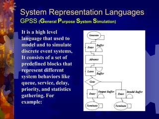
Petri Net
It is a low level
language that used to
model and to simulate
discrete-event and
continuous-time
systems, It consists only
of tow predefined-
blocks [Place and
Transition], which are
enough to represent
very complex systems.
For example:

14. AI Techniques
 Neural Network : Modeling and
Learning
 Fuzzy System: Decision Making
 Genetic Algorithm: Optimization
Artificial Intelligent (AI) techniques, are used
to efficiently solve many control system
problems:

15. Main Topics
 Goals
 Background
 Achievements
 Related Tools
 Conclusion and Future Work

16. Achievements
 Techniques and Algorithms
1. Mixed simulation technique
2. Generalized Petri Net Model
3. Generalized Fuzzy System Object Model
4. New Matrix Based Language
5. Generalized model for dead time element
 CAD Tool
 Libraries
 AI Components
 Applied Examples

17. 1.Mixed simulation technique
more …
 Support both continuous-time and/or discrete-
event-driven systems
 Based on discrete event simulation, and modified
for the continues-time system case
 Support Object Oriented Programming Model
(Blocks are Isolated from each others, communication
established by events, Blocks data and functionality are
encapsulated within the block/object)
 Successfully used within the tool to simulate
systems represents by:
 Input/output block diagram
 Petri-Nets
 GPSS

18. 1.Mixed simulation technique
Continuous Time Simulation Technique
Start
Initialization
E=R-C Summer
If E>0 Then M=1
ELSE M=0 On-Off
L=L+T*(K*M-L) / T Lag
Time = Time + T Time Update
Time<ET
L
Time

19. 1.Mixed simulation technique
Discrete event Simulation Technique
Start
Initialization
Get Top Event
Time<ET
Time = Event Time
Process Event
Event 1
Event 2
Event 3
-
-
Event Time QL
Item Arrive 0.4 0
Begin Processing 0.4 0
Item Arrive 0.5 1
Item Arrive 0.6 2
End Processing 0.8 2
Begin Processing 0.8 1

20. 1.Mixed simulation technique
The Simulator use modified discrete event
simulation technique to perform both
simulation types.

21. 1.Mixed simulation technique
K1 K2t
OP
E1
Time = T1
E2
Time = T1
Current Time = T1
Event Queue
E1 at T1
Event Queue
E1 at T1
Event Queue
E2 at T1
Event Queue

22. 1.Mixed simulation technique
K1 K2t
OP
E 2
Time = T1
E 3
Time = T1
E 1
Time= T1+T
Current Time = T1
Event Queue
E2 at T1
E1 at T1+ T
Event Queue
E2 at T1
E1 at T1+ T
Event Queue
E3 at T1
E1 at T1+ T
Event Queue
 E1 at T1+ T

23. 1.Mixed simulation technique
Rules
• Elements activate whenever event
arrive
•Dynamic element doesn't activate
twice at the same time
• Simulation starts from inputs
• Time will advance only if the
schematic contains dynamic inputs
1 Event Queue (Time=T-T)
 E (Step Input) at T
4 Event Queue (Time=T)
 E (Sum2) at T
E (Step Input) at T+ T
2 Event Queue (Time=T)
 E (Sum1) at T
E (Step Input) at T+ T
5 Event Queue (Time=T)
 E (Controller2) at T
E (Step Input) at T+ T
6 Event Queue (Time=T)
 E (Lag1) at T
E (Step Input) at T+ T
7 Event Queue (Time=T)
 E (Dead Time) at T
E (Step Input) at T+ T
8 Event Queue (Time=T)
 E (Sum2) at T
E (Lag2) at T
E (Step Input) at T+ T
9 Event Queue (Time=T)
 E (Lag2) at T
E (Controller2) at T
E (Step Input) at T+ T
10 Event Queue (Time=T)
 E (Controller2) at T
E (Sum1) at T
E (Scope) at T
E (Step Input) at T+ T
12 Event Queue (Time=T)
 E (Scope) at T
E (Controller1) at T
E (Step Input) at T+ T
13 Event Queue (Time=T)
 E (Controller1) at T
E (Step Input) at T+ T
3 Event Queue (Time=T)
 E (Controller1) at T
E (Step Input) at T+ T
14 Event Queue (Time=T)
 E (Step Input) at T+ T
11 Event Queue (Time=T)
 E (Sum1) at T
E (Scope) at T
E (Step Input) at T+ T
15 Event Queue (Time=T+T)
 E(Sum1) at T+T
E (Step Input) at T+ 2xT

24. 2.Generalized Petri Net Model
 Support Following Petri-Nets types
 Discrete and Continuous (constant or variable
speed)
 Deterministic and Stochastic
 Autonomous and Non-Autonomous (T or P timed)
 Priority
 Any hybrid combination of above
 Integrated within the simulator

25. 2. Generalized Petri Net Model
Structure
Place
Transition
Place
In Arc
Out Arc
Place: Type, Marking, Delay Type, Delay,
Capacity, Sampling-Time
Transition:Type, Delay Type, Delay,
Semantic Type, Sampling Time, Velocity,
Speed Type, Firing Quantity
In Arc: Weight Type, Weight, Inhibited,
Priority Level, Priority Weight
Out Arc: Weight Type, Weight

26. 2. Generalized Petri Net Model
Proposed Event Graph
Place
Transition
Place
1
234
56
7
8
10
8
9
9
Numb
er
Event Name Direction
1 Init Place  Discrete or Continuous Place
2 Enable
Transition
Discrete Place  Discrete or Continuous Transition
Continuous Place  Discrete Transition
3 Reserve Marks Discrete Transition  Discrete or Continuous Place
Continuous Transition  Discrete Place
4 Remove Marks Discrete Transition  Discrete or Continuous Place
Continuous Transition  Discrete Place
5 Pre-Add Marks Discrete Transition  Discrete or Continuous Place
Continuous Transition  Discrete Place
6 Add Marks Discrete Transition  Discrete or Continuous Place
Continuous Transition  Discrete Place
7 Release Marks Discrete Place  Discrete Place
8 Place Time
Update
Continuous Place  Discrete Place
9 Transition
Time Update
Continuous Transition  Continuous Transition

27. 3. Generalized Fuzzy System Object Model
Features
 General
 Complexity wrapping
 Fast
 Multilevel of manipulation
 Easy to use
 Accuracy control

28. 3. Generalized Fuzzy System Object Model
Features: General
Supported Memberships: Triangle, Trapezoidal, Pi, Beta,
Gaussian, Delta, Linear, Crisp, Points (General Case)
Support Hedge operation on memberships : Slightly,
Extremely, Very, Somewhat, Generally, Below, Positively,
Above, Close, Vicinity, About
Support logical operation (AND,OR, Not) on memberships:
Supported AND methods:Zadeh, Mean, Meansqr, Meansqrt,
Product, Boundedprod, Invproduct, Logproduct,
Drasticprod, Boundedsum, Yager, Dubois Prade
Support following De-Fuzzification methods : COG, COA,
Average Momentum, Absolute Momentum, Delta COG
Support alpha cut, rule weighting, rule inversion

29. 3. Generalized Fuzzy System Object Model
Features: Complexity Warping
CFuzzySystem
Array of Input Variables
Array of Output Variables
Inference Object
CFuzzyVariable
Array of Memberships
CFuzzyMembership
CFuzzyRule
CFuzzyInference
Array of Rules

30. 3. Generalized Fuzzy System Object Model
Features: Fast
All three representation are used, by default all memberships
are converted to discrete representation when the fuzzy
system starts the on-line mode

31. 4. New Matrix Based Language
Power Matrix Script
Why?
 Most of operation are base on matrices
 Complexity of calculation
 Give the user the ability to customize
the tool. And to define new elements
and operations

32. 4. New Matrix Based Language
Power Matrix Script
Specification
 Language with all structured languages features
 Global variables, variables, constants
 Control statement [If, for, while, switch]
 Functions, subroutines
 Support recursive calling
 Variables and Constants are matrices or vectors
 Support all matrix operations

33. 4. New Matrix Based Language
Power Matrix Script
Feature
 Support 9 data types [all C data types + complex],
this feature doesn't supported by Matlab script
 Perform automatic data conversion
 Function support any number of input and output
arguments
 High Error protection against user mistakes
 Libraries can be extended by functions and
subroutines and exported C functions
 Automatically detect libraries
 Integrated with the simulator
 Encapsulated within single object

34. 5. Generalized model for dead time element
Definition
Dead Time

35. 5. Generalized model for dead time element
Programming Model
1 2 3 N
Input OutputModel 1
Model 2
Slow
Fast
Large memory usage
Doesn't support dynamic dead time value,
required memory re-allocation for each change

36. 5. Generalized model for dead time element
Proposed Model
• Represented with ring with movable starting point
• Buffer size is limited with certain value

37. 5. Generalized model for dead time element
Proposed Model
M: maximum length of actual buffer L: Current length of actual buffer
1 2 N3 I I+R
Unused Area
1 2 L MJ
Theoretical Buffer
Actual Buffer
N>L
L=R*L
Unused Area
M
Theoretical Buffer
Actual Buffer
1 2 NI
1 2 LJ
N=L

38. 5. Generalized model for dead time element
Proposed Model

39. CAD Tool
Visual environment enable the user to plane and
to design different control problems
Features
• One environment support all simulation operations (design, test,
debugging, developing)
• Visual and follow standard GUI of CAD tools
• Extendable with libraries and routines, with automatic library detector
• Support parallel operations
• Custom interface, based on user needs
• Protected against user errors, and Easy to use

40. CAD Tool – Schematic Editor

41. CAD Tool – Power Matrix Interpreter

42. CAD Tool
System representation within the tool
Connection 1 Element
Source = summer
Destination = PID
Connection n Element
System
Elements Array
Summer
Scope
Step Input
PID
Motor
Summer Element
Scope Element
Step Input Element
PID Element
Connection 1
Connection …
…
ID = 716
Type = 102
Library = “Control”
P = 100
I = 2
D = 0
Connection 1 Element
ID = 611
Type = 11
Library = “Common”
Source = summer
Destination = PID
Motor Macro Element
System
System “Motor”
ID = 718
Type = 70
Library = “Common”
Elements
Dead Time
Lag
…

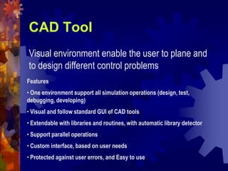
43. CAD Tool
Detail tool structure
element i sub-system j
Schematic Editor
System
Simulator
Power-Matrix Script Interpreter
Libraries Viewer Object Inspector
Value1P1
P2 Value2
… ...
Loaded
Libraries
Lib1 Lib2 Lib n
Library
Element
Definition
Environment Variables
Definition
Environment
Variables
Runtime Variables
Control CenterCommand Line Interpreter
Syntax/Script Editor
A = [1 2 3]
B= C + D
IF(A>PI/2)
B=C+D;
END;
A
Others

44. Libraries
 Input/Output blocks library
 Inputs
 Outputs
 Control Elements
 Linear
 Non-Linear
 Hardware
 Math
 GPSS
 Petri Net
120 Element

45. AI Techniques
 Fuzzy Logic system
 Neural system
 Genetic

46. Applied Examples
1. Adaptive Fuzzy-PID Control
2. Fuzzy Control For Liquid Level Process
3. Fuzzy Control For Inverted Pendulum
Process
4. Traffic System Design Using Petri-Nets
5. Production Line of CDs Factory
6. Model-Based Fuzzy-PID Control

47. Applied Examples
1. Adaptive Fuzzy-PID Control
Fuzzy System
PID
d/dt
P I D
Error
e
e.
Control

48. Applied Examples
1. Adaptive Fuzzy-PID Control
System: First order + Dead Time
Conventional PID tuning for optimal response
Optimization Methods
• Iterative Search
•  Hill Climbing
• Random Hill Climbing
• Simulated Annealing
• Genetic
System  Td=5, Tc=5, K=5
Optimal PID  P=466.406, I=7.71484, D=1.69385  IAE=7.73928

49. Applied Examples
1. Adaptive Fuzzy-PID Control
Schematic

50. Applied Examples
1. Adaptive Fuzzy-PID Control
Results

51. Applied Examples
1. Adaptive Fuzzy-PID Control
Schematic to study the effect of parameter change within
certain range

52. Applied Examples
1. Adaptive Fuzzy-PID Control
Results

53. Applied Examples
2. Fuzzy Control For Liquid Level Process
System

54. Applied Examples
2. Fuzzy Control For Liquid Level Process
Schematic

55. Applied Examples
2. Fuzzy Control For Liquid Level Process
Fuzzy Settings

56. Applied Examples
2. Fuzzy Control For Liquid Level Process
Results

57. Applied Examples
2. Fuzzy Control For Liquid Level Process
Modified Fuzzy Control
If Level is Very Very Low Then Valve is Open-fast2
If Level is Very Very High Then Valve is Close-fast2

58. Applied Examples
2. Fuzzy Control For Liquid Level Process
Results

59. Applied Examples
3. Fuzzy Control For Inverted Pendulum Process
Process

60. Applied Examples
3. Fuzzy Control For Inverted Pendulum Process
Fuzzy Settings
Fuzzy
Angle
Velocity
Force

61. Applied Examples
3. Fuzzy Control For Inverted Pendulum Process
Schematic
H=D;
T(1)=H(2); //velocity
T(2)=(4*(f-mu*H(2))-
1.5*bm*g*sin(2*H(3))+4*bm*L*H(4)^2*sin(H(3)))/(4*(TM+bm)-
3*bm*(cos(H(3)))^2); //acceleration
T(3)=H(4); //angular velocity
T(4)=(3/(4*L))*(g*sin(H(3))-T(2)*cos(H(3)));//angular acceleration
…K2=T;
…K3=T;
…K4=T;
D=D+(K1+K2*2+K3*2+K4)*(DELTAT/6);
x=D(1); v=D(2); a=D(3); w=D(4);
Inverted Pendulum Model using Power Matrix Script

62. Applied Examples
3. Fuzzy Control For Inverted Pendulum Process
Results

63. Applied Examples
3. Fuzzy Control For Inverted Pendulum Process
Traffic System Components - Petri Net Model
Road Segment

64. Applied Examples
4. Traffic System Design Using Petri-Nets
Traffic System Components - Petri Net Model
PI Intersection

65. Applied Examples
4. Traffic System Design Using Petri-Nets
Traffic System Components - Petri Net Model
U-Turn

66. Applied Examples
4. Traffic System Design Using Petri-Nets
Traffic System Components - Petri Net Model
Square

67. Applied Examples
4. Traffic System Design Using Petri-Nets
System Model
2 traffic Intersections using Squares

68. Applied Examples
4. Traffic System Design Using Petri-Nets
System Model
2 traffic Intersections using U-Turns

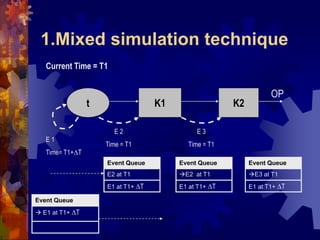
69. Applied Examples
4. Traffic System Design Using Petri-Nets
Results
Input car generators [T=10,W=1] for each road
Simulation Time: 10000 second
Results:
Model 1 Model 2
Average Queue Length 3.067 0.1748
Average System Capacity 61.77 15.5
Case Study 1: Low Traffic
Input car generators [T=2,W=1] for each road
Simulation Time: 10000 second
Results:
Model 1 Model 2
Average Queue Length 466 0.8722
Average System Capacity 7500 77.9308
Case Study 2: Heavy Traffic

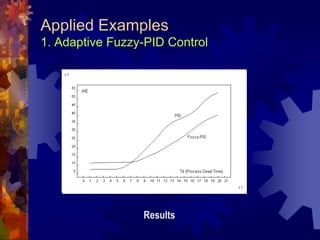
70. Applied Examples
5. Production Line of CDs Factory
• Factory contains following production lines
• [Disk, Upper Cover, Down Cover, Holder ] Lines
• Assembly and Covering Line produce complete CD
• Packaging into small Boxes Line
• Packaging into Large Cartons Line
• Lines separated by buffers
• Input martial [Plastic Powder, Tin , Plastic Cover, Labels,
Small Boxes, Large Cartons] is stored in input buffers

71. Applied Examples
5. Production Line of CDs Factory
GPSS - Model

72. Applied Examples
5. Production Line of CDs Factory
Case Study "Study the effect of Tin level update quantity"
Tin level update = 100 Kg/Day
Simulation Time 300,000 second (about 3 days)
Results:
Average Level of Tin material: 46.244
Maximum Level of Tin material: 200
Average Length of Tin Covering Queue: 547.147
Maximum Length of Tin Covering Queue: 2700
Production Rate: 9039/300000  108.468 CD/hour
Case Study

73. Applied Examples
5. Production Line of CDs Factory
Case Study "Study the effect of Tin level update quantity“
Tin level update = 100 Kg/Day
Rate of change of Tin material level
= - 0.0020544 kg/sec
The required level update every date
= 0.0020544*24*60*60 = 177.5 KG
Conclusion

74. Applied Examples
5. Production Line of CDs Factory
Case Study "Study the effect of Tin level update quantity“
Tin level update = 177.5 Kg/Day

75. Applied Examples
5. Production Line of CDs Factory
Case Study "Study the effect of number of assembling units
on production "
Number of assembling machines = 1
Simulation Time = 100000
Results
Average Assembling Queue Length = 1316.32
Maximum Assembling Queue Length = 2699
CDs Production Rate = 977/100000 à 844.128 CD/hour
Case Study
Assembling Queue input rate = -0.00983607
Assembling Queue output rate = 0.0724138
Required number of assembling machines
= 0.0724138/0.00983607 = 7.36
Conclusion

76. Applied Examples
6. Model-Based Fuzzy-PID Control
PID System
Model 1 (Td=1)
Model 2 (Td=5)
Model 3 (Td=10)
Model
Selector
Fuzzy PID
For large Td
Fuzzy PID
For small Td
Optimal P, I, D
For Td=5
MUX
-

77. Applied Examples
6. Model-Based Fuzzy-PID Control
Identification Schematic
Process (Td=1,5,10)

78. Applied Examples
6. Model-Based Fuzzy-PID Control
Control Loop Schematic

79. Applied Examples
6. Model-Based Fuzzy-PID Control
Results

80. Main Topics
 Goals
 Background
 Achievements
 Related Tools
 Conclusion and Future Work

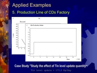
81. Related Tools
GPSS-World
Simulator supports only standard GPSS language
 Standard
 Very fast simulation
 Based on command mode interface [not visual]
 Supported programming language is very week
 Simulation Output in text format, no graphs, no
direct analysis can be applied
Advantage
Disadvantage

82. Related Tools
SIMULINK
Represents any continuous time system using
Input/Output block diagram
 Interact with Matlab functionality
 Support Fuzzy and Neural systems
 Does not support Discrete Event Systems
 Support only floating point operations even
logical operation
Advantage
Disadvantage

83. Topics
 Goals
 Background
 Achievements
 Related Tools
 Conclusion and Future Work

84. Development Environment
 Programming Environment: Microsoft Visual C++
version 6.0
 Operating System: Windows 95,98,2000 or NT4
 CPU: AMD K6-III 450 with 1 MB cash and 128 MB
RAM
 Programming Language: C/C++
 Aided tools: Matlab and SIMULINK version 4 and
5.1, GPCC/PC, GPCC world, QNET neural network
simulator, Neurosolulton simulator, FULDIC Fuzzy
simulator, and Matlab Fuzzy Component.

85. Software Specification
 Source Code Size: above 50,000 line of code, 700
file, 600 class, 150 exported function, 2,5 MB pure
code, 309 MB project development size
 Software Components: one executable file, 3 static
libraries, 6 dynamic libraries
 Tool Size: 3.9 MB for the complete released running
version with libraries.
 Minimum Hardware Requirements: 32 MB ram, 5
MB disk space, Pentium 133 or any compatible
processor.

86. Conclusion
 Both Continuous-Time and Discrete-Event systems can be
simulated using Event-Driven Simulation with special treatment
for Continuous-Time systems
 Standard interface for libraries and components increase the
ability for extension
 Object-Oriented programming simplify the development, and
produce modular code, easy to understand and easy to extend
 Using internal interpreter gives the ability to define un-limited
number of custom elements and functions. On another hand it
slow down the simulation
 The simulator succeeds to implement all proposed simulation
languages, in spite they used different simulation techniques
 Using internal interpreter increase the capabilities of GPSS
language. It increases the ability to generate more statistics and
to perform more complicated calculations

87. Future Work
 This version supports non-interactive continues-time elements
(input and outputs supposed to be buffered), and there is a need
to support interactive continuous-time elements (electronic
elements)
 There is a need for a module that exports and imports
standard simulation language file formats. Especially Matlab
and Simulink file formats
 Current version of the simulator does not support distributed
simulation, for that, there is a need for modified technique that
support this type
 Simulation language can be extended by (Colored Petri Net,
State Flow)
 There is a need for native compiler for Power Matrix script

88. Thank You

89. Integrated Tools for the Analysis
and Design of Intelligent Control
System
Submitted by:
Eng. Mohamed Ali Ali Sobh
Supervised By:
Prof. Mohamed Abd El-hamid Sheirah
Ain Shams University, Faculty of Engineering
Computer and Systems Engineering Department