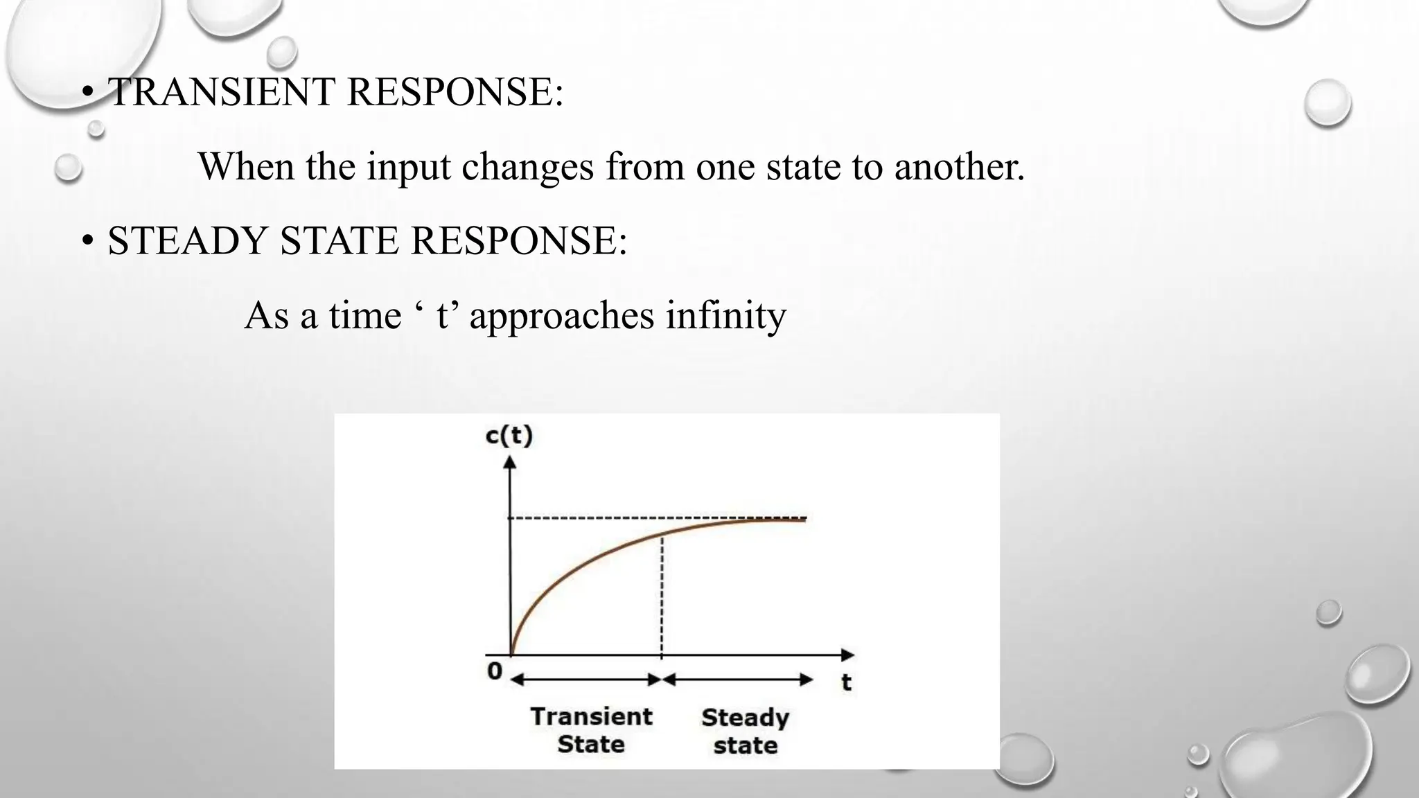
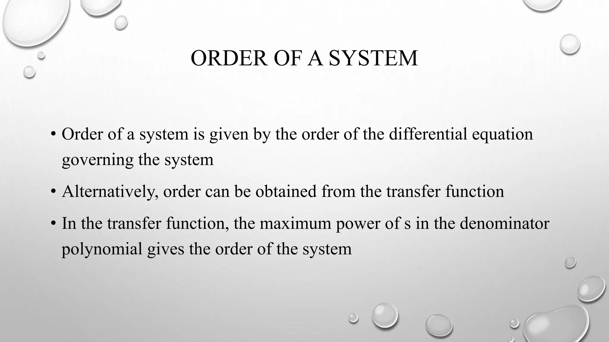
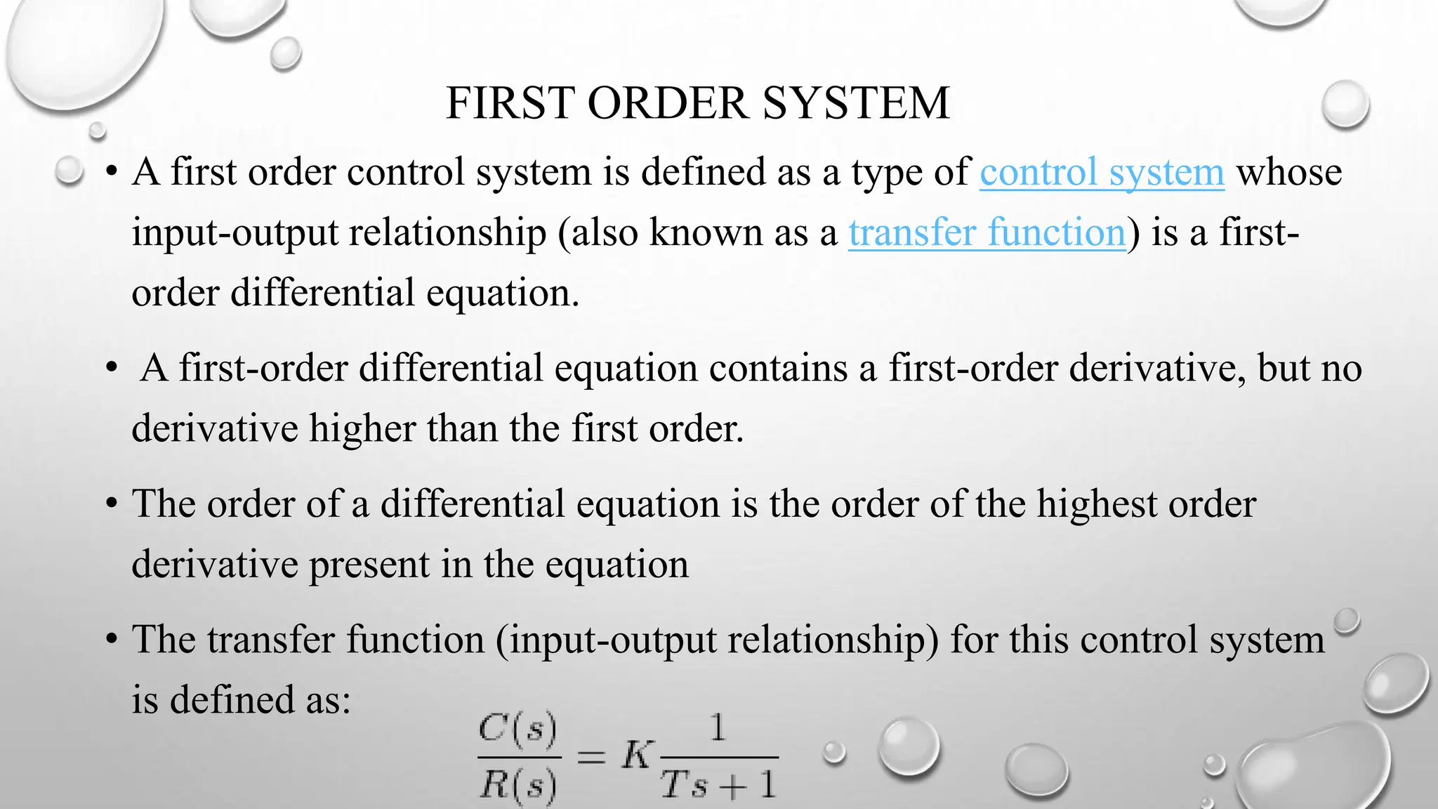
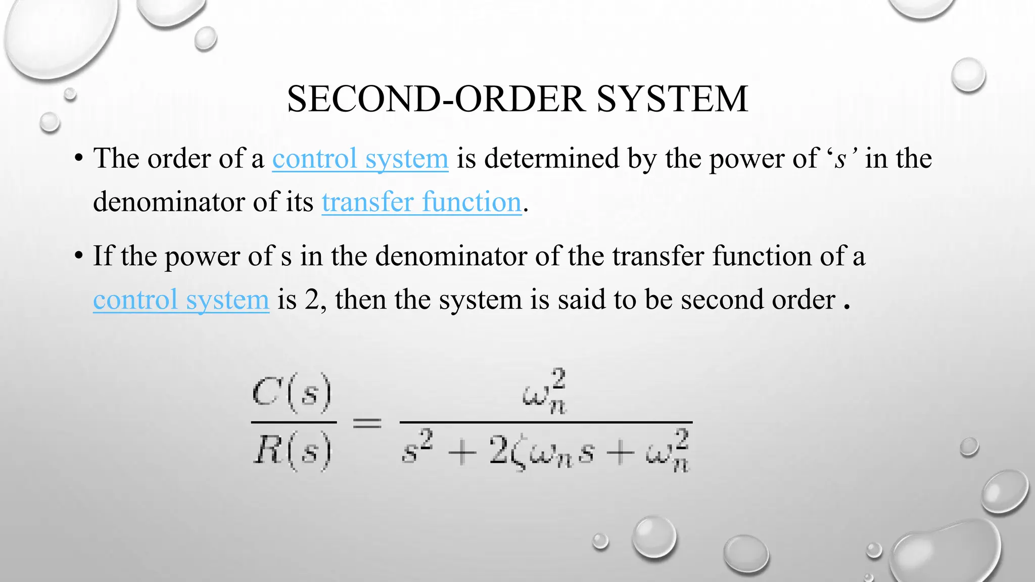
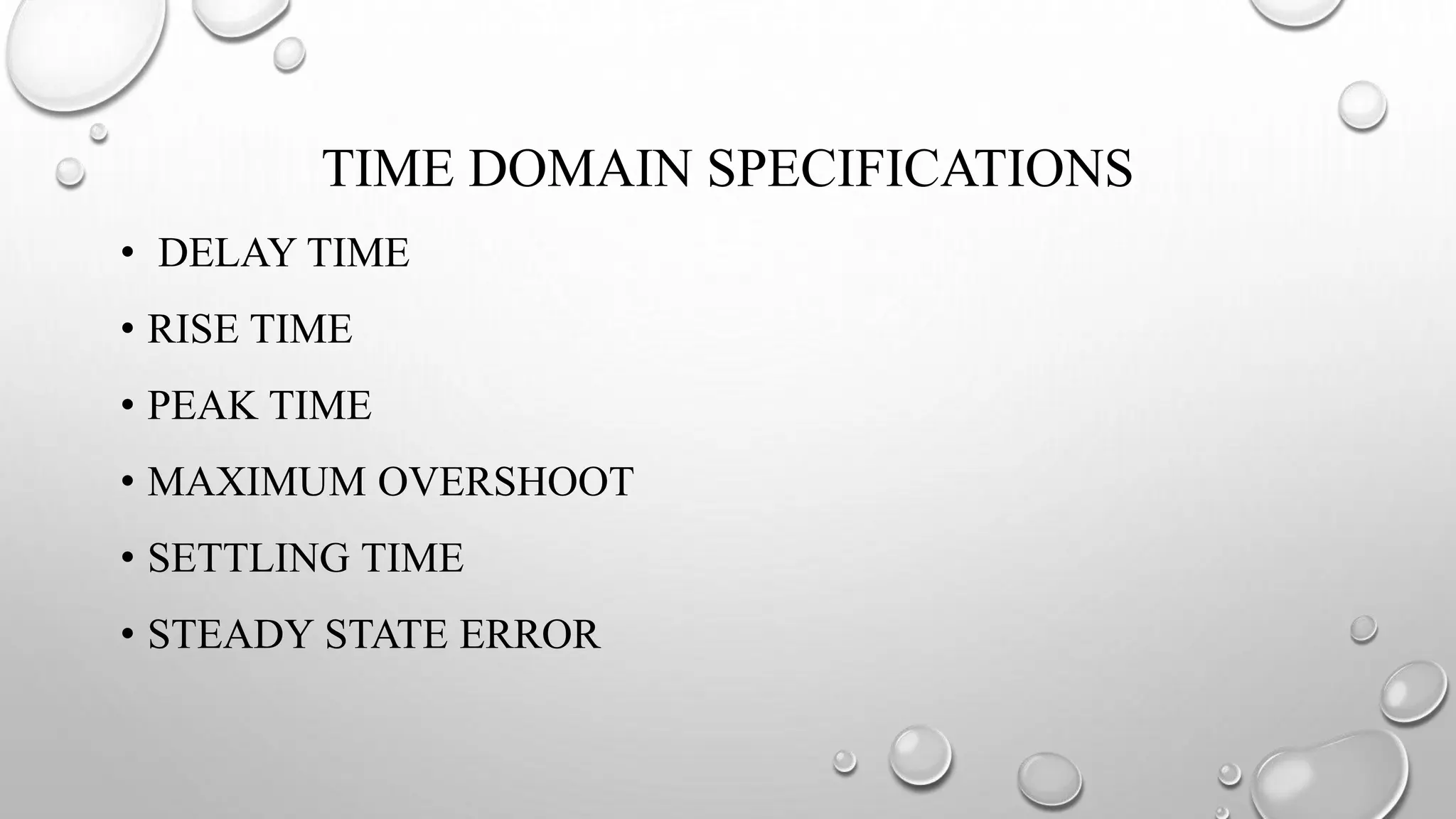
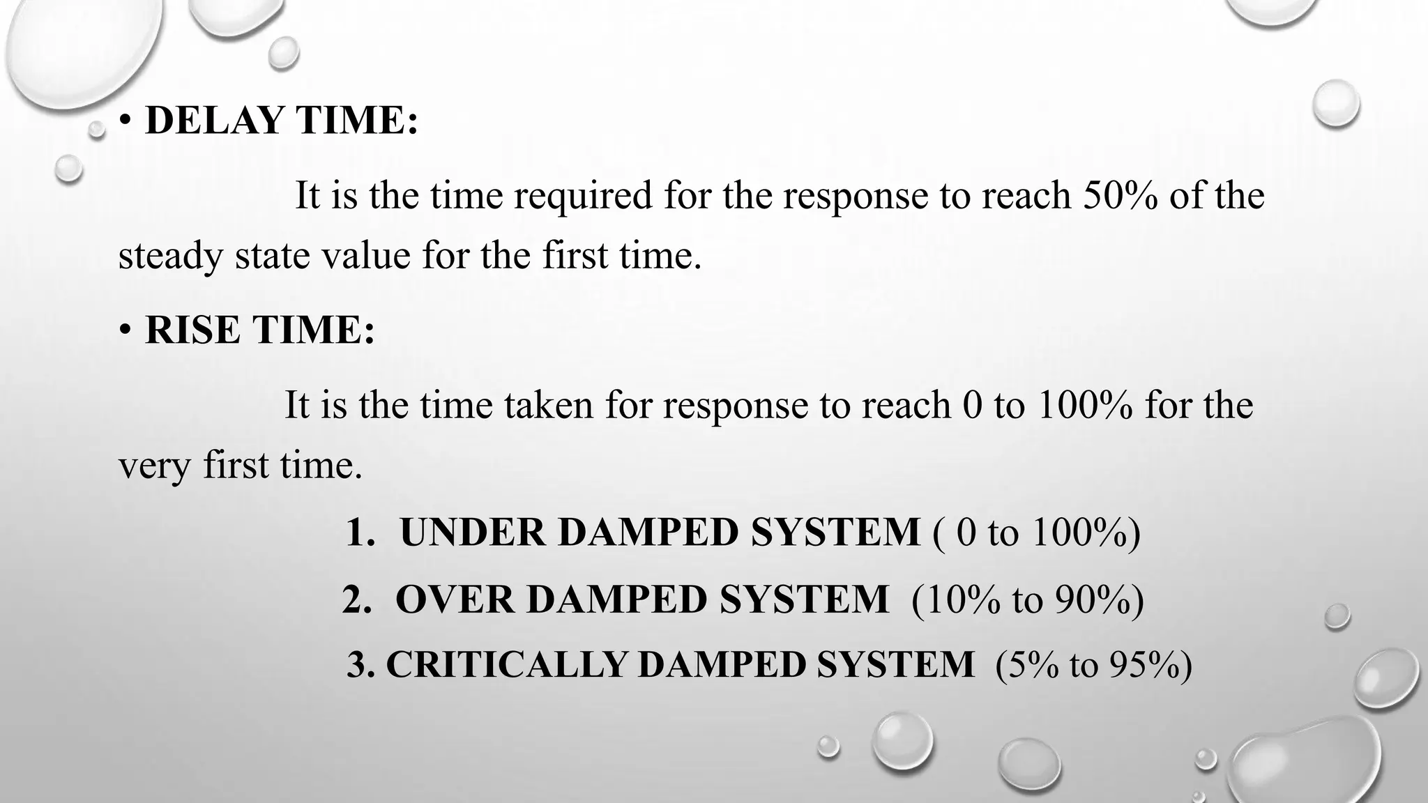
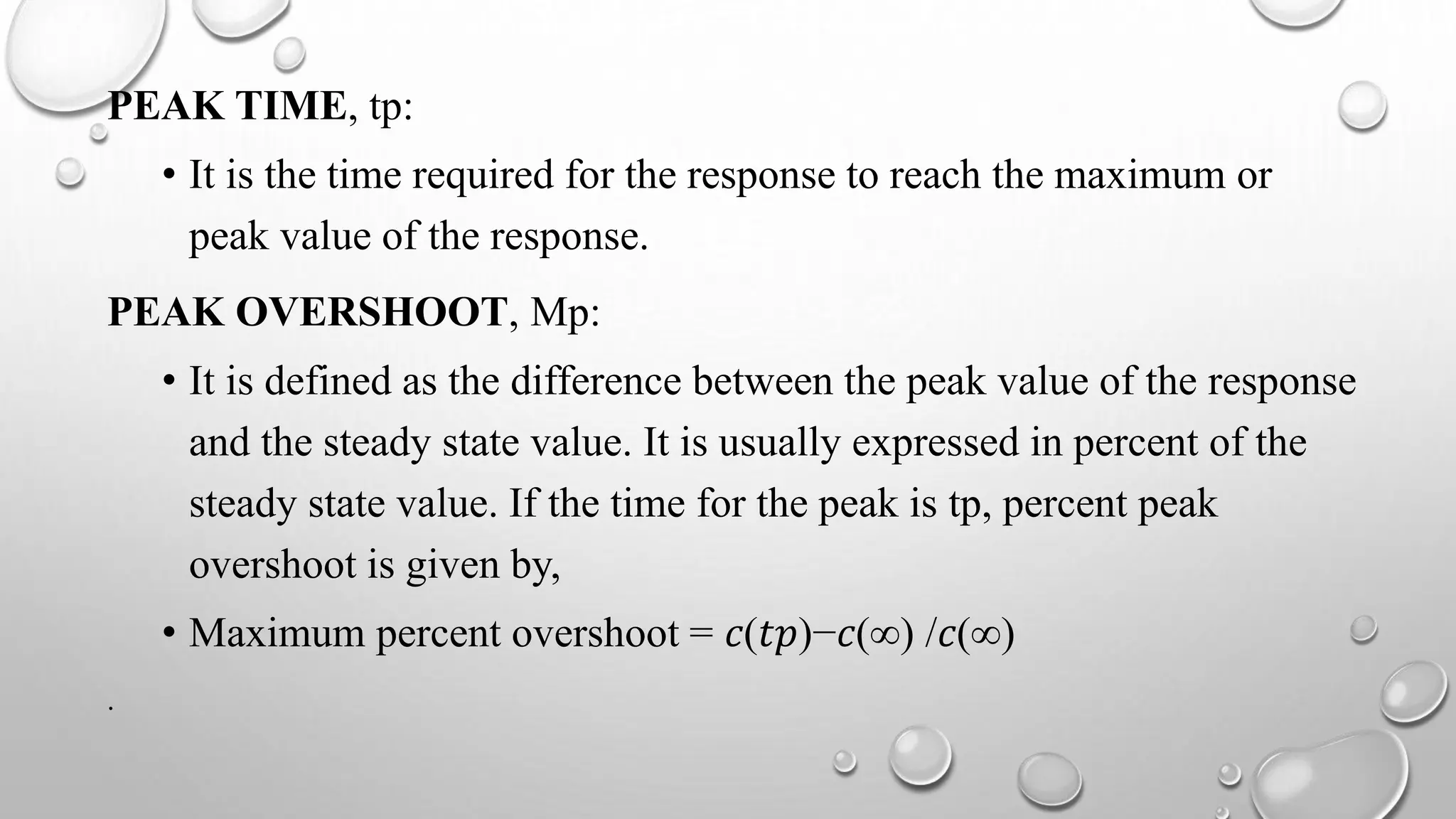
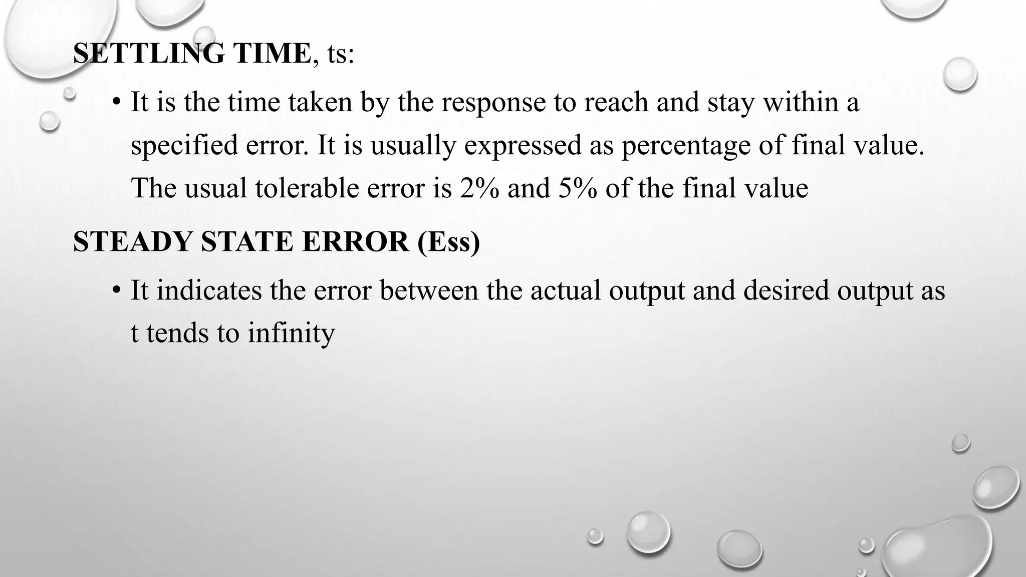
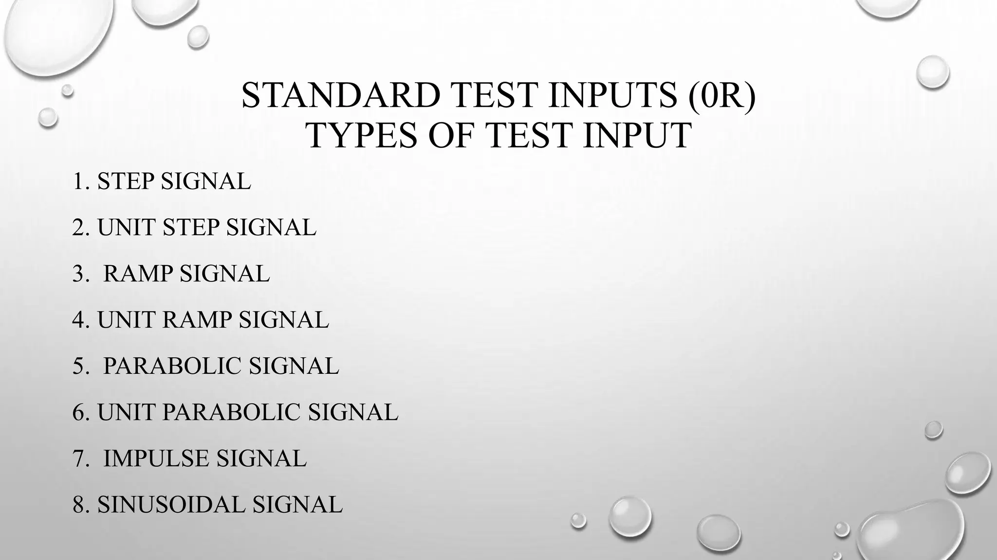
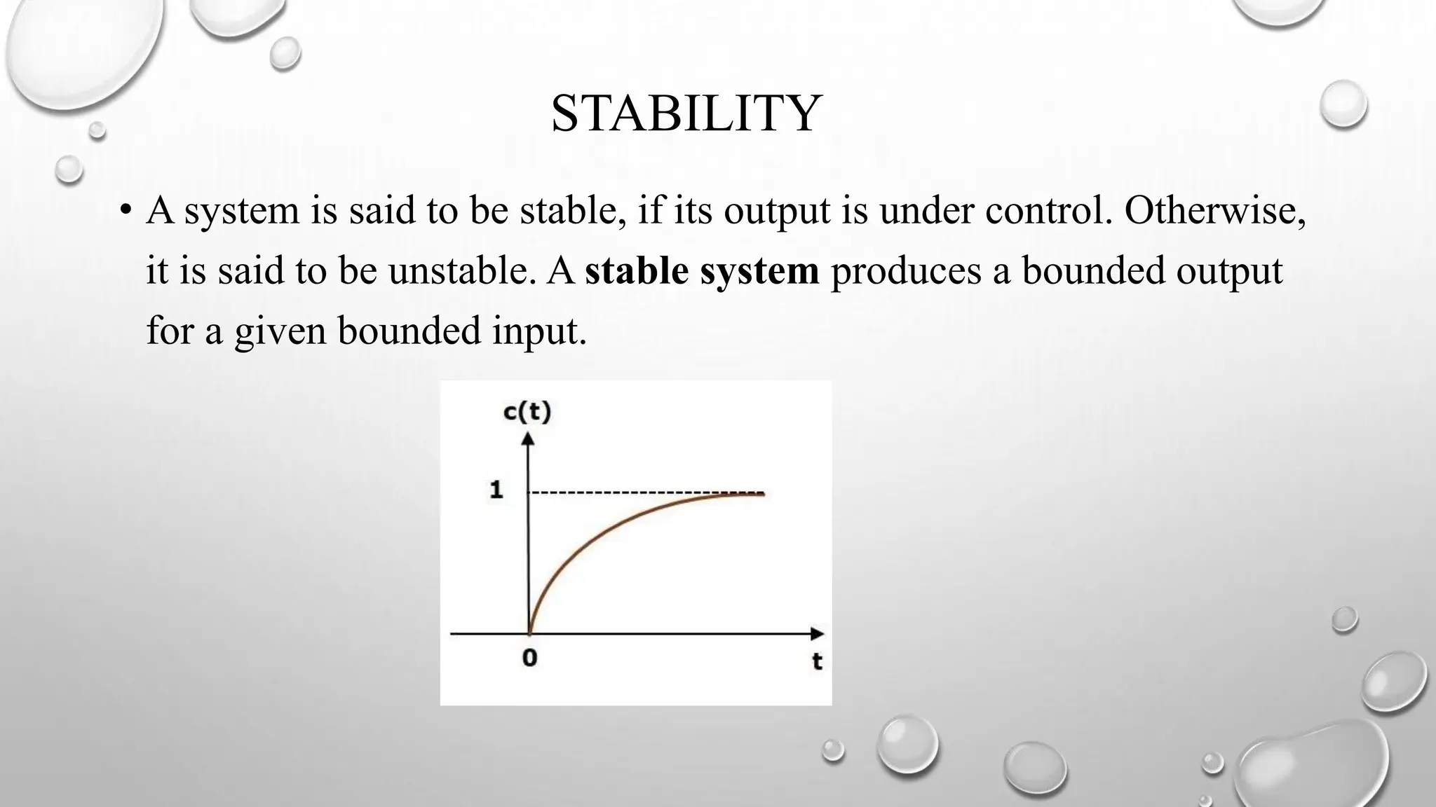
This document discusses various concepts related to time response analysis and stability of control systems. It defines the transient and steady state response of a system. It describes first and second order systems, and specifies their transfer functions and order. It outlines different time domain specifications used to characterize response, such as rise time, settling time, overshoot. It also covers standard test inputs, stability types, and classification of systems as absolutely, conditionally and marginally stable based on their stability properties.

1. EE3503-CONTROL SYSTEMS
UNIT -II
BY
MRS. R.RAMYA .ME,
AP/EEE
SSMIET.DINDIGUL

2. TIME RESPONSE
• The time response of the system is the output of the closed loop
system as a function of time
• It is Denoted by c(t)
• It consists of two parts
1. Transient response
2. Steady state response

3. • TRANSIENT RESPONSE:
When the input changes from one state to another.
• STEADY STATE RESPONSE:
As a time ‘ t’ approaches infinity

4. FIRST AND SECOND ORDER SYSTEM
RESPONSE
TRANSFER FUNCTION
• It is the ratio of Laplace transform of output to Laplace transform of
input with zero initial conditions.
• One of the types of modeling a system
• Differential equation is obtained
• Laplace transform is applied to the equation assuming zero initial
conditions

5. ORDER OF A SYSTEM
• Order of a system is given by the order of the differential equation
governing the system
• Alternatively, order can be obtained from the transfer function
• In the transfer function, the maximum power of s in the denominator
polynomial gives the order of the system

6. FIRST ORDER SYSTEM
• A first order control system is defined as a type of control system whose
input-output relationship (also known as a transfer function) is a first-
order differential equation.
• A first-order differential equation contains a first-order derivative, but no
derivative higher than the first order.
• The order of a differential equation is the order of the highest order
derivative present in the equation
• The transfer function (input-output relationship) for this control system
is defined as:

7. SECOND-ORDER SYSTEM
• The order of a control system is determined by the power of ‘s’ in the
denominator of its transfer function.
• If the power of s in the denominator of the transfer function of a
control system is 2, then the system is said to be second order .

8. TIME DOMAIN SPECIFICATIONS
• DELAY TIME
• RISE TIME
• PEAK TIME
• MAXIMUM OVERSHOOT
• SETTLING TIME
• STEADY STATE ERROR

9. • DELAY TIME:
It is the time required for the response to reach 50% of the
steady state value for the first time.
• RISE TIME:
It is the time taken for response to reach 0 to 100% for the
very first time.
1. UNDER DAMPED SYSTEM ( 0 to 100%)
2. OVER DAMPED SYSTEM (10% to 90%)
3. CRITICALLY DAMPED SYSTEM (5% to 95%)

10. PEAK TIME, tp:
• It is the time required for the response to reach the maximum or
peak value of the response.
PEAK OVERSHOOT, Mp:
• It is defined as the difference between the peak value of the response
and the steady state value. It is usually expressed in percent of the
steady state value. If the time for the peak is tp, percent peak
overshoot is given by,
• Maximum percent overshoot = 𝑐(𝑡𝑝)−𝑐(∞) /𝑐(∞)
.

11. SETTLING TIME, ts:
• It is the time taken by the response to reach and stay within a
specified error. It is usually expressed as percentage of final value.
The usual tolerable error is 2% and 5% of the final value
STEADY STATE ERROR (Ess)
• It indicates the error between the actual output and desired output as
t tends to infinity

12. STANDARD TEST INPUTS (0R)
TYPES OF TEST INPUT
1. STEP SIGNAL
2. UNIT STEP SIGNAL
3. RAMP SIGNAL
4. UNIT RAMP SIGNAL
5. PARABOLIC SIGNAL
6. UNIT PARABOLIC SIGNAL
7. IMPULSE SIGNAL
8. SINUSOIDAL SIGNAL

13. STEP SIGNAL
• The step signal is a signal whose value changes from zero to A at t=0
and remains constant at A for t>0.
• The step signal resembles an actual steady input to a system. A special
case of step signal is unit step in which A is unity.

14. RAMP SIGNAL
• The ramp signal is a signal whose value increases linearly with time
from an initial value of zero at t=0.
• The ramp signal resembles a constant velocity input to the system. A
special case of ramp signal is unit ramp signal in which the value of A
is unity.

15. PARABOLIC SIGNAL
• In parabolic signal, the instantaneous value varies as square of the
time from an initial value of zero at t=0.
• The sketch of the signal with respect to time resembles a parabola. The
parabolic signal resembles a constant acceleration input to the system.
• A special case of parabolic signal is unit parabolic signal in which A is
unity

16. IMPULSE SIGNAL
• A signal of very large magnitude which is available for very short
duration is called impulse signal.
• Ideal impulse signal is a signal with infinite magnitude and zero
duration but with an area of A.
• The unit impulse signal is a special case, in which A is unity.

17. STABILITY
• A system is said to be stable, if its output is under control. Otherwise,
it is said to be unstable. A stable system produces a bounded output
for a given bounded input.

18. TYPES OF SYSTEMS BASED ON STABILITY
We can classify the systems based on stability as follows.
• Absolutely stable system
• Conditionally stable system
• Marginally stable system

19. ABSOLUTELY STABLE SYSTEM
• If the system is stable for all the range of system component values,
then it is known as the absolutely stable system.
• The open loop control system is absolutely stable if all the poles of
the open loop transfer function present in left half of ‘s’ plane.
• Similarly, the closed loop control system is absolutely stable if all
the poles of the closed loop transfer function present in the left half
of the ‘s’ plane.

20. CONDITIONALLY STABLE SYSTEM
• If the system is stable for a certain range of system component
values, then it is known as conditionally stable system.
MARGINALLY STABLE SYSTEM
• If the system is stable by producing an output signal with constant
amplitude and constant frequency of oscillations for bounded input, then
it is known as marginally stable system