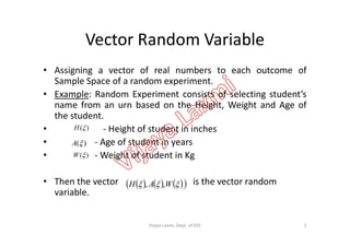
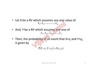
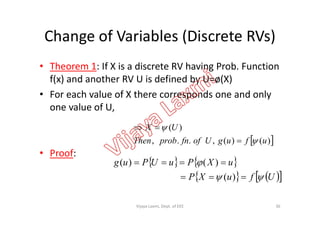
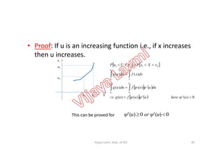
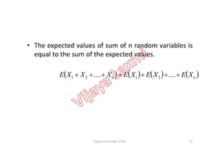
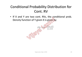
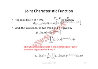
1) A vector random variable assigns a vector of real numbers to each outcome of a random experiment. An example is selecting a student's name from an urn based on their height, weight, and age. This would make the vector random variable equal to (height, age, weight).
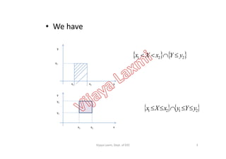
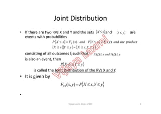
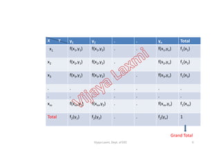
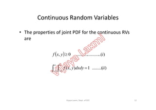
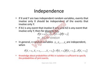
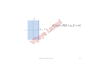
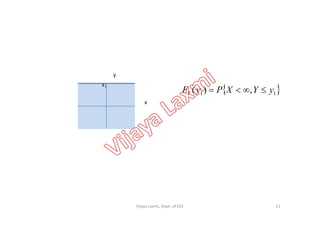
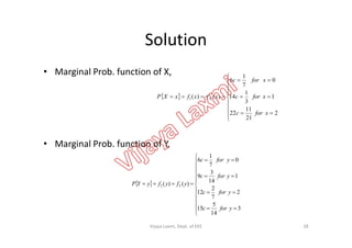
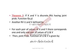
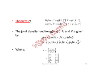
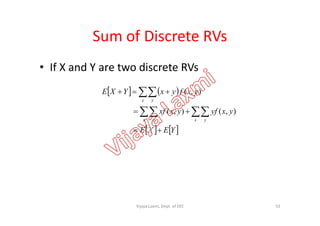
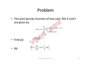
2) For discrete random variables X and Y, their joint probability distribution is defined as the probability that X assumes a value less than or equal to x, and Y assumes a value less than or equal to y. This can be written as P(X≤x, Y≤y).
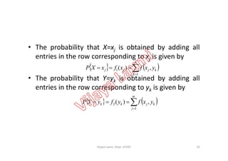
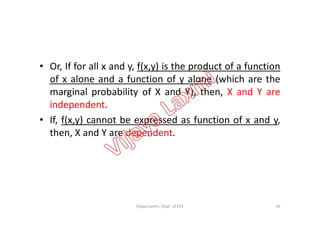
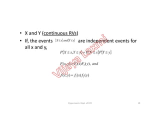
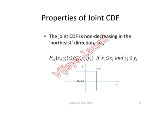
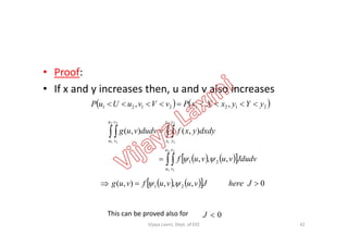
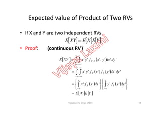
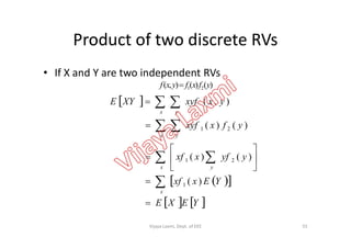
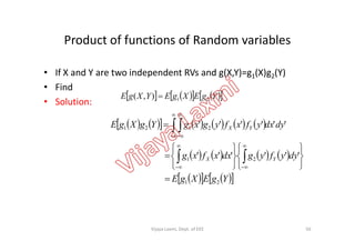
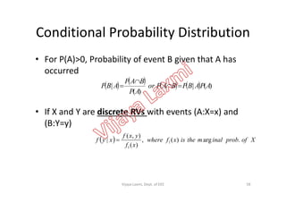
3) If the joint probability distribution of X and Y can be written as the product of the marginal probability distributions of X and

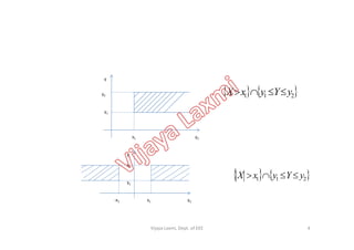
![Correlation and Covariance of Two RVs
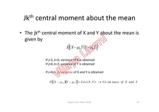
• The jkth joint moment of two RVs X and Y is defined
as
kj
YX
kjKj
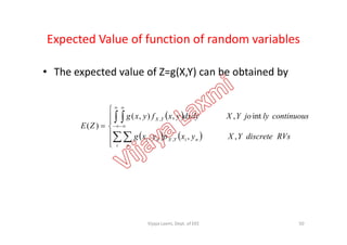
ContinuouslyjoYandXFordxdyyxfyxYXE int,,
i n
niYX
k
n
j
i RVsdiscreteYandXyxpyx ,,
If j=0, moments of Y are obtained
If k=0, moments of X are obtained
If j=k=1, E[XY] gives the correlation of X and Y
IF E[XY]=0, X and Y are orthogonal
66Vijaya Laxmi, Dept. of EEE](https://image.slidesharecdn.com/moduleiiisp-180416041134/85/Module-iii-sp-66-320.jpg)
![Covariance of Two RVs
YEXEYEXEXYE
YEXEXYE
YXXYE
YXEYXCov
YXXY
YXXY
YX
2
),(
YEXEXYE
YEXEYEXEXYE
2
Hence,
Cov(X,Y)=E[XY], if either of the RVs has mean value equal to zero
68Vijaya Laxmi, Dept. of EEE](https://image.slidesharecdn.com/moduleiiisp-180416041134/85/Module-iii-sp-68-320.jpg)
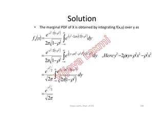
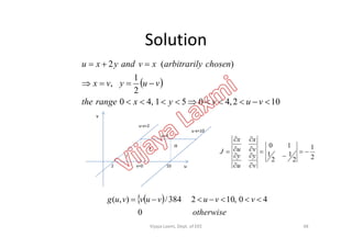
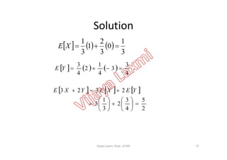
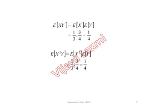
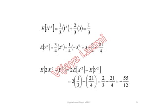
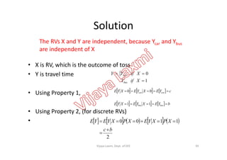
![Solution
1
2.2.
0
2
0
2
dyeydxex
YEXEYXE
yx
1
4 22
dxdyexyeXYE yx
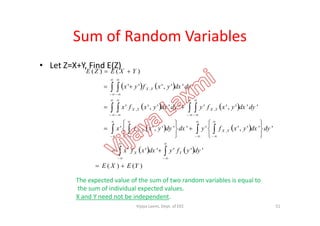
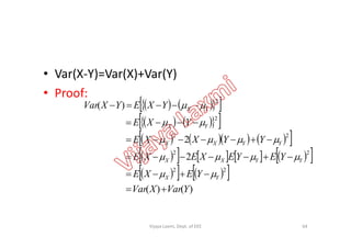
Check E[X+Y]=E[X]+E[Y]
E[XY]=E[X]E[Y]
70
4
4
0 0
22
dxdyexyeXYE yx
122
0
22
0
2222
dyeydxexYXE yx
Vijaya Laxmi, Dept. of EEE](https://image.slidesharecdn.com/moduleiiisp-180416041134/85/Module-iii-sp-70-320.jpg)
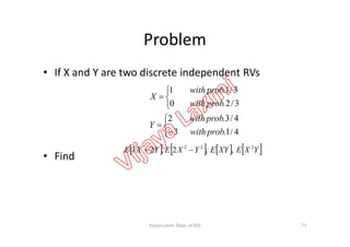
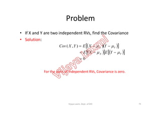
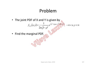
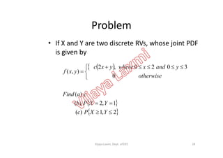
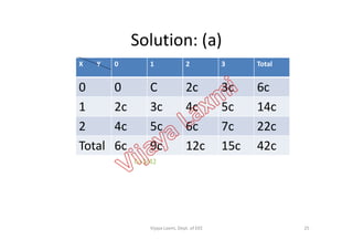
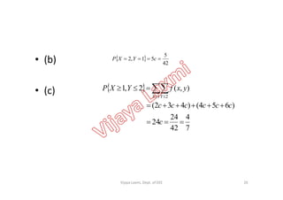
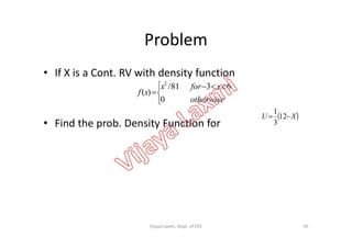
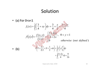
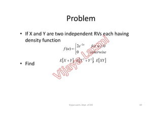
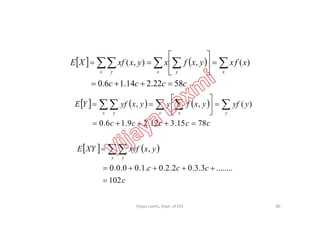
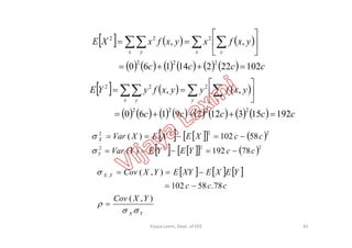
![Problem
• If X and Y are two discrete RVs, whose joint density function is
given by
• Find E[X], E[Y], E[XY], E[X2], E[Y2], Var(X), Var(Y), Cov(X,Y) and
otherwise
yxforyxcyxf
0
30,202),(
• Find E[X], E[Y], E[XY], E[X2], E[Y2], Var(X), Var(Y), Cov(X,Y) and
correlation coeff.
78Vijaya Laxmi, Dept. of EEE](https://image.slidesharecdn.com/moduleiiisp-180416041134/85/Module-iii-sp-78-320.jpg)
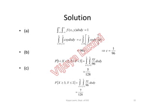
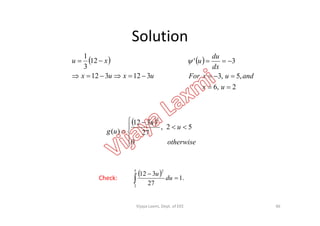
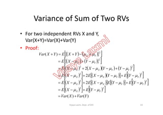
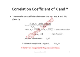
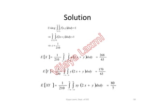
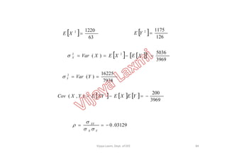
![Problem
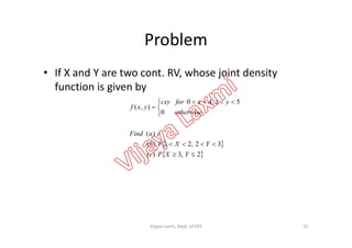
• If X and Y are two Cont. RVs
• Find (a) c
• (b) E[X]
otherwise
yxforyxc
yxf
0
50,622
,
• (c) E[Y]
• (d) E[XY]
• (e) E[Y2]
• (f) Var(X)
• (g) Var(Y)
• (h) Cov(X,Y)
• (i) Correlation Coeff.
82Vijaya Laxmi, Dept. of EEE](https://image.slidesharecdn.com/moduleiiisp-180416041134/85/Module-iii-sp-82-320.jpg)
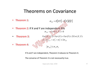
![
02
4
1
2
1
2
0
2
0
dSin
dCosSinCosSinEXYE
Since E[X]=E[Y]=0, X and Y are uncorrelated
Uncorrelated but dependent Random Variables
87Vijaya Laxmi, Dept. of EEE](https://image.slidesharecdn.com/moduleiiisp-180416041134/85/Module-iii-sp-87-320.jpg)
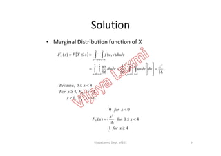
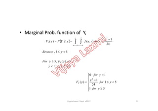
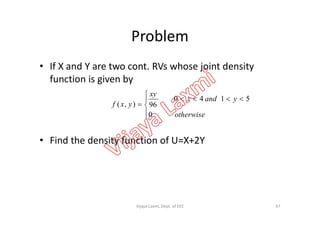
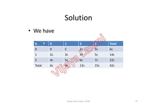
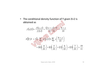
![Problem
• If X and Y are two RVs whose density function is
given by
otherwise
yxforyxcyxf
0
30,202,
• Find E[Y|X=2]
91Vijaya Laxmi, Dept. of EEE](https://image.slidesharecdn.com/moduleiiisp-180416041134/85/Module-iii-sp-91-320.jpg)
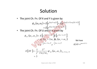
![Problem
• If U and V are independent zero mean, unit
variance Gaussian RV, and
• X=U+V and Y=2U+V
• Find the joint ch. Fn of X and Y and find E[XY]• Find the joint ch. Fn of X and Y and find E[XY]
103Vijaya Laxmi, Dept. of EEE](https://image.slidesharecdn.com/moduleiiisp-180416041134/85/Module-iii-sp-103-320.jpg)
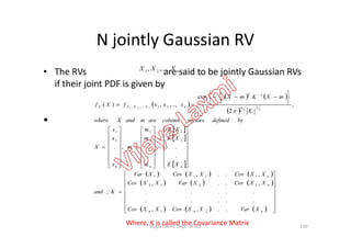
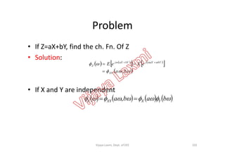
![Problem
• The PDF for jointly Gaussian RVs is given by
16168
3
8
3
16
3
4
2
1
,
22
2
1
,
yx
xy
yx
YX eyxf
• Find E[X], E[Y], Var(X), Var(Y) and Cov(X,Y)
106Vijaya Laxmi, Dept. of EEE](https://image.slidesharecdn.com/moduleiiisp-180416041134/85/Module-iii-sp-106-320.jpg)