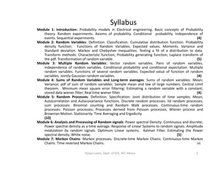
This document outlines the syllabus and objectives for a course on probability and random processes for electrical engineering. The syllabus covers topics like probability models, random variables, multiple random variables, sums of random variables, random processes, analysis of random signals, Markov chains, and related mathematical concepts. The objectives are to describe and analyze various probabilistic concepts and random signals, and to design filters and estimators for random systems and processes.

1. 1Vijaya Laxmi, Dept. of EEE, BIT, Mesra

2. Syllabus
Module 1: Introduction: Probability models in Electrical engineering. Basic concepts of Probability
theory. Random experiments. Axioms of probability. Conditional probability. Independence of
events. Sequential experiments. (4)
Module 2: Random Variables: Definition. Classification. Cumulative distribution function. Probability
density function. Functions of Random Variables. Expected values. Moments. Variance and
Standard deviation. Markov and Chebyshev inequalities. Testing a fit of a distribution to data.
Transform methods: Characteristic function; Probability generating function; Laplace transform of
the pdf. Transformation of random variable. (5)
Module 3: Multiple Random Variables: Vector random variables. Pairs of random variables.
Independence of random variables. Conditional probability and conditional expectation. Multiple
random variables. Functions of several random variables. Expected value of function of random
variables. Jointly Gaussian random variables. (4)
Module 4: Sums of Random Variables and Long-term averages: Sums of random variables: Mean;
Variance; pdf of sum of random variables. Sample mean and law of large numbers. Central LimitVariance; pdf of sum of random variables. Sample mean and law of large numbers. Central Limit
theorem. Minimum mean square error filtering: Estimating a random variable with a constant;
stored data wiener filter; Real time wiener filter. (4)
Module 5: Random Processes: Definition. Specification: Joint distribution of time samples; Mean;
Autocorrelation and Autocovariance functions. Discrete random processes: iid random processes;
sum processes: Binomial counting and Random Walk processes. Continuous-time random
processes: Poisson processes; Processes derived from Poisson processes; Wiener process and
Brownian Motion. Stationarity. Time Averaging and Ergodicity.
(10)
Module 6: Analysis and Processing of Random signals: Power spectral Density: Continuous and discrete;
Power spectral density as a time average. Response of Linear Systems to random signals. Amplitude
modulation by random signals. Optimum Linear systems. Kalman Filter. Estimating the Power
spectral density. White noise. (5)
Module 7: Markov Chains: Markov processes. Discrete-time Markov Chains. Continuous-time Markov
Chains. Time reversed Markov Chains. (4)
2Vijaya Laxmi, Dept. of EEE, BIT, Mesra

3. Books:
Text Book
1. Probability and random Processes for Electrical Engineering- A. Leon-Garcia
Reference Books
2. Probabaility, Random Variables and Stochastic Processes- A. Papoulis & S. U. Pillai.
3. Random Signals- K. Sam Shanmugan & A.M Breipohl.3. Random Signals- K. Sam Shanmugan & A.M Breipohl.
3Vijaya Laxmi, Dept. of EEE, BIT, Mesra

4. Course Objectives
This course enables the students :
• To describe and classify different types of random variables,
random processes, probability density function and
cumulative distribution function
• To estimate statistical properties of random variables and
random processes such as expected value, variance, standardrandom processes such as expected value, variance, standard
deviation and correlation functions.
• To evaluate autocorrelation functions for given power spectral
density, correlate the mean square error of any system with
the correlation functions and analyse the response of linear
system to random inputs.
• To design real time wiener filter, stored data Wiener filter and
Kalman filter for any system.
4Vijaya Laxmi, Dept. of EEE, BIT, Mesra

5. Course Outcomes
After the completion of this course, students will be able to:
• Enumerate properties of probability density function,
cumulative distribution function, correlation functions and
power spectral density of a random process
• Describe different types of random variable and random
processesprocesses
• Calculate expected value, variance, standard deviation and
correlation functions of a random variable and random
process.
• Analyse the response of linear system to random inputs.
• Design a Wiener and Kalman filter for a system and compare
with classical filters
5Vijaya Laxmi, Dept. of EEE, BIT, Mesra

6. MODULE 1
6Vijaya Laxmi, Dept. of EEE, BIT, Mesra

7. Probabilistic models in Electrical and Computer
Engineering
Mathematical models are used as tools in analysis and design.
This is based on certain factors:
• Based on making choices from various alternatives.
• Choices are based on criteria such that cost, reliability and
performanceperformance
• Decisions are made based on estimates that are obtained
using different models.
7Vijaya Laxmi, Dept. of EEE, BIT, Mesra

8. Mathematical model
• This is used when observational phenomenon has
measurable properties.
• It consists of a set of assumptions about how a system or
physical process works.
• These assumptions are stated in the form of mathematical• These assumptions are stated in the form of mathematical
relations involving the important parameters and variables of
the system.
• Experiments carried out determines ‘givens’ in the
mathematical relations and solution allows to predict the
measurements.
8Vijaya Laxmi, Dept. of EEE, BIT, Mesra

9. Deterministic model
• An experiment carried out determine the exact outcome of
the experiment and the solution of the set of mathematical
equations specifies the exact outcome of the experiment.
• Example: Circuit theory
9Vijaya Laxmi, Dept. of EEE, BIT, Mesra

10. Probabilistic models
• Random experiment: In this case the outcome varies in an
unpredictable manner, when the experiment is repeated
under the same conditions.
• Deterministic models are not appropriate for random
experiment.experiment.
• Example: selection of a ball from a box containing three balls
labeled 0,1 and 2.
• In this case, the outcome of the experiment is a number from
a set .
Where S is the sample space.
 2,1,0S
10Vijaya Laxmi, Dept. of EEE, BIT, Mesra

11. Outcome of Random experiment
11Vijaya Laxmi, Dept. of EEE, BIT, Mesra

12. Statistical Regularity
• This states that the averages obtained in long
sequences of repetitions (trials) of random
experiment consistently yield approximately the
same value.
Let N (n), N (n), N (n) are the number of times outcomes are• Let N0(n), N1(n), N2(n) are the number of times outcomes are
balls 0, 1 and 2
12Vijaya Laxmi, Dept. of EEE, BIT, Mesra

13. Relative frequency
• The relative frequency is given by,
• Statistical regularity means, fk(n) varies less and less
   
trialsofnumbertheisnwhere
n
nN
nf k
k
,

• Statistical regularity means, fk(n) varies less and less
about a constant value as n is made large
  koutcomeofyprobabilittheispnf kk
n


lim
13Vijaya Laxmi, Dept. of EEE, BIT, Mesra

14. • The relative frequencies fk(n) converges to 1/3 as
• If one more ball is placed on the box numbered as 0
Probability of outcome 0 is 2/4
Probability of outcome 1 & 2 is ¼
• Hence, the conditions under which a random experiment is
n
• Hence, the conditions under which a random experiment is
performed, determine the probability of outcome of an
experiment.
14Vijaya Laxmi, Dept. of EEE, BIT, Mesra

15. Properties of Relative Frequencies
• Suppose for a random experiment, there are K
possible outcomes, the sample space is given by
 KS ....,,2,1,0
....,,3,2,11)(0.2
....,,3,2,1)(0.1

 k
Kkfornf
KkfornnN
 
  1.4
.3
....,,3,2,11)(0.2
1
1







K
k
k
K
k
k
k
nf
nnN
Kkfornf
Property 3 shows that the sum of number of occurances of all
Possible outcomes must be n.
Property 4 shows that the sum of all relative frequencies equals n,
and is obtained by dividing both sides of property 3 by n. 15Vijaya Laxmi, Dept. of EEE, BIT, Mesra

16. • Suppose the event is ‘even numbered ball selected’
• Then
• Relative frequency,
     nNnNnNE 20 
         nfnf
n
nNnN
nfE 20
20



• So, we can say that if ‘A and B occurs’ then C be the event
• And
n
     
     nfnfnf
nNnNnN
BAC
BAC


16Vijaya Laxmi, Dept. of EEE, BIT, Mesra

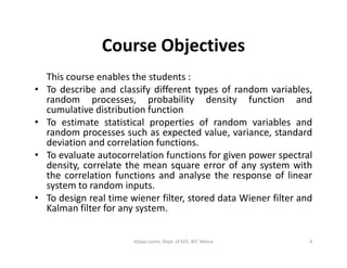
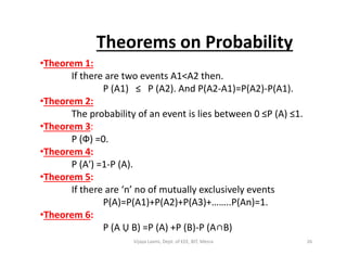
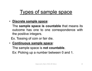
17. Axioms on Probability
It supposes
• A random experiment has been defined and a set S of all
possible outcomes has been identified
• A class of subsets of S called events has been specified
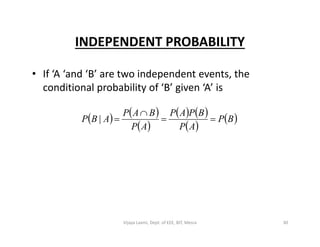
• Each event a has been assigned a number P[A]• Each event a has been assigned a number P[A]
 
 
     BorAPBPAP
eouslysimuloccurcannotBandAIf
SP
AP



tan.3
1.2
10.1
17Vijaya Laxmi, Dept. of EEE, BIT, Mesra

18. Building a Probabilistic Model
This involves
• Defining the random experiment
• Specifying the set S of all possible outcomes and events of interest
• Specifying a probability assignment from which probabilities of all events
of interest can be computed
• Ex. Telephone conversation to determine whether a speaker is currently
speaking or silent. An speaker in general remains active (speaking) for 1/3
of time and remain silent for 2/3 (listening to others)
This problem is similar to selecting a ball from a box containing two
white balls (silent) and one black ball (active).
18Vijaya Laxmi, Dept. of EEE, BIT, Mesra

19. Problem
• Find the probability that 24 speakers out of 48
independent speakers are active simultaneously.
• Solution:• Solution:
The problem is same as finding the probability of
selecting 24 black balls in 48 independent trials in
the previous experiment.
19Vijaya Laxmi, Dept. of EEE, BIT, Mesra

20. Example
• A communication system is required to transmit 48
simultaneous conversations from city A to city B.
• The speech is first converted into voltage signals which are
digitized and bundled into packets of information that
corresponds to 10ms signals.corresponds to 10ms signals.
20Vijaya Laxmi, Dept. of EEE, BIT, Mesra

21. Stochastic processes
• Random experiments which has outcome as a function of time or
space
Examples:
• Speech recognition system: speech signal in converted to voltage
waveforms
• Image processing system: the intensity of image varies over a• Image processing system: the intensity of image varies over a
rectangular region
• Queuing system: the number of customers varies with time
• Arrival of telephone calls at an exchange
• Arrival of a customer to a service station
• Breakdown of a component of some system
• Number of printing errors in a book
21Vijaya Laxmi, Dept. of EEE, BIT, Mesra

22. BASIC CONCEPTS OF PROBABILITY THEORY
• RANDOM EXPERIMENT:
A random experiment is an experiment in which the
outcome varies in an unpredictable fashion, when the
experiment is repeated under the same conditions.
• SAMPLE SPACE:
The sample space S of a random experiment is defined as
the set of all possible outcomes.
22Vijaya Laxmi, Dept. of EEE, BIT, Mesra

23. Types of sample space
• Discrete sample space:
The sample space is countable that means its
outcome has one to one correspondence with
the positive integers.the positive integers.
Ex. Tossing of coin or fair die.
• Continuous sample space:
The sample space is not countable.
Ex: Picking up a number between 0 and 1.
23Vijaya Laxmi, Dept. of EEE, BIT, Mesra

24. EVENT
• EVENT: The event occurs if and only if the outcome
of the experiment ξ is in the subset.
Ex: Select a ball from box numbered from 1 to 50.
• Certain event:
It consists of all outcomes hence always occurs.It consists of all outcomes hence always occurs.
• Null event/impossible event):
It contains no outcome and it never occur.
• Elementary event:
Event from a discrete sample space that consists of a
single outcome.
24Vijaya Laxmi, Dept. of EEE, BIT, Mesra

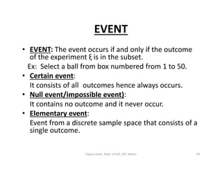
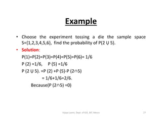
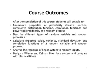
25. PROBABILITY:
It is the measure of uncertainty of occurrence of an event or
chance of probability of occurrence of an event.
THE AXIOMS OF PROBABILITY:
Axiom 1: 0 ≤ P [A]
Axiom 2: P[S] =1Axiom 2: P[S] =1
Axiom 3:
For any no. of mutual exclusively events A1, A2, A3 …An. in the
class C.
P (A1 Ụ A2 Ụ A3………………… Ụ An)=
P(A1)+P(A2)+P(A3)+……..P(An).
25Vijaya Laxmi, Dept. of EEE, BIT, Mesra

26. •Theorem 1:
If there are two events A1<A2 then.
P (A1) ≤ P (A2). And P(A2-A1)=P(A2)-P(A1).
•Theorem 2:
The probability of an event is lies between 0 ≤P (A) ≤1.
•Theorem 3:
P (Ф) =0.
Theorems on Probability
P (Ф) =0.
•Theorem 4:
P (A′) =1-P (A).
•Theorem 5:
If there are ‘n’ no of mutually exclusively events
P(A)=P(A1)+P(A2)+P(A3)+……..P(An)=1.
•Theorem 6:
P (A Ụ B) =P (A) +P (B)-P (A∩B)
26Vijaya Laxmi, Dept. of EEE, BIT, Mesra

27. Example
• Choose the experiment tossing a die the sample space
S={1,2,3,4,5,6}, find the probability of P(2 Ụ 5).
• Solution:
P(1)=P(2)=P(3)=P(4)=P(5)=P(6)= 1/6
P (2) =1/6, P (5) =1/6P (2) =1/6, P (5) =1/6
P (2 Ụ 5). =P (2) +P (5)-P (2∩5)
= 1/6+1/6=2/6.
Because(P (2∩5) =0)
27Vijaya Laxmi, Dept. of EEE, BIT, Mesra

28. CONDITIONAL PROBABILITY
• If A and B are two events A, B, such that P (A)>0, the
conditional probability of B of A is given by
   
 AP
BAP
ABP

|   0APprovided
 AP
28Vijaya Laxmi, Dept. of EEE, BIT, Mesra

29. Example
• Tossing a die and the event is odd and is less then ‘4’.
• Solution:
P(1)=P(2)=P(3)=P(4)=P(5)=P(6)= 1/6
P (A) = P (1) +P (3) +P (5) =3/6.
P (B) = P (1) +P (2) +P (3) =3/6P (B) = P (1) +P (2) +P (3) =3/6
P (A∩B) = P (1) +P (3) =2/6.
   
 AP
BAP
ABP

|
3/2
6/3
6/2

29Vijaya Laxmi, Dept. of EEE, BIT, Mesra

30. INDEPENDENT PROBABILITY
• If ‘A ‘and ‘B’ are two independent events, the
conditional probability of ‘B’ given ‘A’ is
   
 
   
 
 BP
AP
BPAP
AP
BAP
ABP 

| 
   
 BP
APAP
ABP |
30Vijaya Laxmi, Dept. of EEE, BIT, Mesra