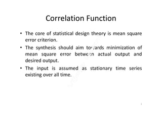
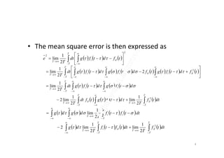
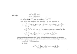
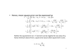
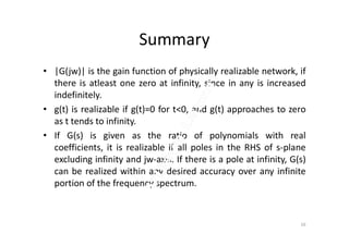
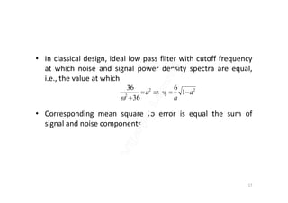
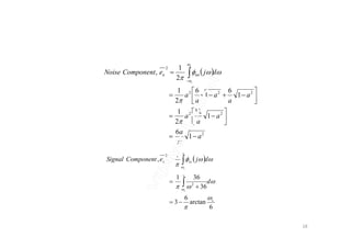
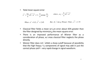
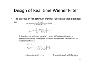
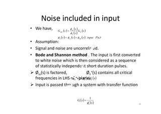
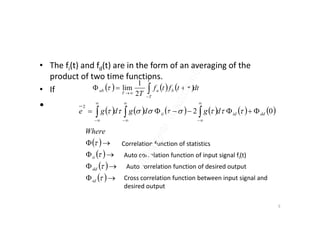
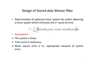
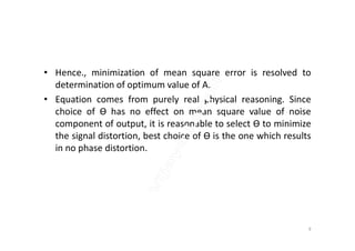
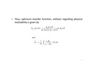
The document discusses correlation functions and their use in designing optimal Wiener filters. It contains the following key points: 1. Correlation functions describe the relationships between input and output signals of a system and include the auto-correlation of the input, auto-correlation of the desired output, and cross-correlation between input and output. 2. The Wiener filter is a linear filter that minimizes the mean square error between the actual and desired filter output. It can be designed by determining the transfer function that results in the lowest mean square error based on the correlation functions. 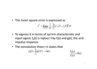3. For a stationary input signal, the optimal Wiener filter transfer function is derived by setting the cross-correlation between the input and

1. Module IV

2. Correlation Function
• The core of statistical design theory is mean square
error criterion.
• The synthesis should aim towards minimization of
mean square error between actual output andmean square error between actual output and
desired output.
• The input is assumed as stationary time series
existing over all time.
2

3. • The mean square error is expressed as
• To express it in terms of system characteristic and
    

T
T
d
T
dttftf
T
e
2
0
2
2
1
lim
• To express it in terms of system characteristic and
input signal, f0(t) is replaced by fi(t) and g(t), the unit
impulse response.
• The convolution theorem states that
      ,0  dtfgtf i  


3
 
 
 sG
sF
sF
i
0

4. • The mean square error is then expressed as
     
2
2
2
1
lim  










T
T
di
T
tfdtfgdt
T
e 
                  














T
T
didii
T
tfdtfgtfdtfgdtfgdt
T
2
2
2
1
lim 
4
       
       
 












T
T
d
T
id
T
T
T
ii
T
T
T
dttf
T
dtfgtfdt
T
dtfgdtfgdt
T
2
2
1
lim
2
1
lim2
2
1
lim


       
       
 














T
T
d
T
d
T
T
i
T
T
T
ii
T
dttf
T
dttftf
T
dg
dttftf
T
dgdg
2
2
1
lim
2
1
lim2
2
1
lim



5. • The fi(t) and fd(t) are in the form of an averaging of the
product of two time functions.
• If
•
     dttftf
T
T
T
ba
T
ab 

 
2
1
lim
           02
2
ddidii dgdgdge  

           02 ddidii dgdgdge   

Correlation function of statistics
Auto correlation function of input signal fi(t)
Auto correlation function of desired output
Cross correlation function between input signal and
desired output
5
 
 
 
 







id
dd
ii
Where

6. Design of Stored data Wiener filter
• Determination of optimum linear system lies within obtaining
a linear system which minimizes the measure of error.
• Assumption:
          

djjGjGjjGe ssdnn



222
2
1
• Assumption:
 The system is linear.
 Time series is stationary.
 Mean square error is the appropriate measure of system
error.
6

7. • The system is given by figure below
System g(t)Input: fi(t)=s(t)+n(t) Output: fo(t)
System g(t)
Tr. Fn G(jw)
PSD: øii(jw)=øii(jw)+ øii(jw) Desired output , fd(t)
7

8. • We have
     
     tftfte
tgtstf
d
dd
0
,*


       
   
 
 



djeAeAjAe ss
jj
dnn
d






 
2
1 2
22
     
     
    
 
iablerealoffunctionsrealareandAboth
eAjGandeAjG dj
dd
j
var

The equation indicates the optimum choice of Ɵ. (if physical realizability condition are neglected).
Since A, Ad, ønn, øss are nonnegative for all values of w, minimum value of integral occurs when
 
d
dd
or
imumisCosAA




,
max2
8
 
   



dCosAAAAA
djASinACosSinjACosAA
ssdddnn
ssddddnn








)(2
2
1
2
1
222
22
  


 

dAAAAAe ssddnn 2
2
1 2222

9. • Hence., minimization of mean square error is resolved to
determination of optimum value of A.
• Equation comes from purely real physical reasoning. Since
choice of Ɵ has no effect on mean square value of noise
component of output, it is reasonable to select Ɵ to minimizecomponent of output, it is reasonable to select Ɵ to minimize
the signal distortion, best choice of Ɵ is the one which results
in no phase distortion.
9

10. • Hence, mean square error can be expressed as
  


 

dAAAAe ssdssdnnss
222
2
2
1
 














































d
A
A
A
A
d
AA
AAAA
ssd
ssd
ssd
nnss
nnss
ssd
nnss
ssd
ssdssdnnss
22
2
2
2222
22
2
1
2
2
1
Neither the squared term nor the last term can be negative for any value of w,
hence minimum value of mean square error occurs when square term is zero.
nnss
ss
dAA




10










 
 





dAA
nnss
ssd
nnss
nnss
2






















 






d
AA
A
nnss
nnssd
nnss
ssd
nnss
2
2
2
1

11. Problem
• Given a filtering problem
   
  TdelaytimewithinputofcomponentsignaleiejG
ajj
Tj
d
nnSS
.,.
,
36
36 2
2










a2
/36Solution:
Now, compare the designed filter with a filter designed by classical theory.
11
 
 
Tj
opt e
aa
a
jG 

 

 222
2
/136
/36Solution:
 
2
222
2
2
min
1
3
/136
/36
2
1
a
a
d
aa
a
e



 





12. • Thus, optimum transfer function, without regarding physical
realizability is given by
   
   
 


 jG
jj
j
jG d
nnss
ss
opt


12




 



dAe
and
d
nnss
nnss
opt
22
2
1
,

13. 1
PSD
øss
wc-wc w
øss
ønn
13

14. Physically Realizable system
• The design theory lies within determination of physically
realizable network which minimizes the mean square error.
Ein Eout
   
 sE
sE
sG
in
out

 sEin
If input is a sine wave, output is also a sine wave of same frequency w1
 
 1
1


jGEE
EjGE
inout
inout


i.e., in passage of signal through the network, the amplitude is multiplied by
|G(jw1)| and phase is advanced by the angle of G(jw1)
14

15. • Physical realizability of the network requires that G(s) be
analytic in RHS of s-plane i.e., if G(s) is the ratio of
polynomials, all poles must lie in the LHS of s-plane.
• The impulse response must be zero for all negative time i.e.,
there must be no output before the application of the input.there must be no output before the application of the input.
15

16. Summary
• |G(jw)| is the gain function of physically realizable network, if
there is atleast one zero at infinity, since in any is increased
indefinitely.
• g(t) is realizable if g(t)=0 for t<0, and g(t) approaches to zero
as t tends to infinity.as t tends to infinity.
• If G(s) is given as the ratio of polynomials with real
coefficients, it is realizable if all poles in the RHS of s-plane
excluding infinity and jw-axis. If there is a pole at infinity, G(s)
can be realized within any desired accuracy over any infinite
portion of the frequency spectrum.
16

17. • In classical design, ideal low pass filter with cutoff frequency
at which noise and signal power density spectra are equal,
i.e., the value at which
22
2
1
6
36
36
a
a
a c 



• Corresponding mean square to error is equal the sum of
signal and noise components.
17

18.  
22
222
2
1
12
2
1
1
6
1
6
2
1
2
1
,
a
a
a
a
a
a
a
a
djeComponentNoise
c
c
nnn












 






2
1
6
2
a
a
a




18
 
6
arctan
6
3
36
361
1
,
2
2
c
sss
d
djeComponentSignal
c
c

















19. • Total mean square error
• Classical filter fields a mean square error about 42% greater than
the filter designed by minimizing the mean square error.
6
arctan
6
31
6 22
c
a
a
e



73.1,sin,
2
eFilterWienergubyBut
2
1
6
, a
a
where c 
45.2,5.0
22
 eaWhen
the filter designed by minimizing the mean square error.
• There is an improved performance of Wiener filter as a
consideration of phase, whereas classical filter neglects the phase
directly.
• Wiener filter does not exhibit a sharp cutoff because of possibility
that the high frequency components of signal may add in just the
correct phase yield a very rapid change in signal waveform.
19

20. Design of Real time Wiener Filter
• The expression for optimum transfer function is then obtained
as,  
   
 


 jG
jj
j
jG d
nnss
ss
opt

)(
 tj
opt e
a
a
jG 

 







 22
2
/36
/36
)(
It describes the optimum transfer function without consideration of
physical realizability. The exponential term is the desired transfer function
in absence of noise.
 
   sT
opt e
aas
a
sG
sj










222
2
/136
/36

One pole in each half of s-plane
20
aapolesTwo /16 2

a   /36

21. • The impulse response for the first term can be obtained as
• The impulse response corresponding to total G (s) in the• The impulse response corresponding to total Gopt(s) in the
above equation delayed by T is now obtained as
21

22. • Regardless of allowable delay, the optimum system is never exactly
physically realizable, optimum impulse response is never zero for all
negative time even though the response for negative time can be made
small (as small as possible) if sufficiently great delay is admitted.
• But, difficulty arises regardless of Gd(jw) because is always a
function of w2 or s2 i.e., poles in both left and right half plane. nnss
ss


function of w2 or s2 i.e., poles in both left and right half plane.
• Only situation in which optimum transfer function is realizable is the trivial
case in which there is no noise and Gd(jw) is itself realizable.
nnss  
22

23. Noise free system
• For a noise free system, n=0 and
• If Gd(jw) corresponds to a nonrealizable network, the
corresponding inverse waveform, the desired impulse
response is not zero for t<0.
    jGjG dopt 
response is not zero for t<0.
• The simplest example is to design a predictor, where desired
output is a prediction of input, i.e.,
• Hence,
   
valuepositivehaveandtimepredictioniswhere
tstfd

 ,
  
 j
opt ejG 
23

24. Bode and Shannon Method
• The approximation of Gopt(jw) by a realizable G(jw) is solved
by Bode and Shannon method, which is as follows:
 Factorize into two components
ss    
     sss
sands
ssssss
ssss


 

   
  
94 2


s
sIf 
 The subsystems can be drawn as
   
  361
94
22



ss
s
sIf ss
24
   
  
   
  61
32
,
61
32





 
ss
s
s
ss
s
s ssss 

25. • Here, m(t) is the white noise. And,
 
 
  1,
1
1  
s
s
sG mm
ss


            
 
   




ss
jsssssmm
ss
j
sGsGjjGjs










1
.
1
11
2
1
• Waveform of m(t) depends on the waveform of s(t), but the
optimum filter is independent of this waveform and depends only
on the power spectrum density or autocorrelation function.
• It is permissible to consider m(t) as a train of closely spaced narrow
random statistically independent pulses. Hence, select transfer
function G2(s) to operate on these pulses to give best prediction of
input signal s(t).
25
 
    


jsssss
ss
ss
j

 



 .

26. • Each of these pulses produces an output proportional to the
impulse response g2(t), hence total output fo(t) is the sum of
all individual responses.
26

27. • The approximate impulse response for the second section of
predictor is
• Mean square error of prediction is the error introduced by
neglecting the pulses of m(t) from t=0 to t= α, if output at t=0 is
considered.
 
 





0,
0,0
2
ttg
t
tg
ss 
    


0
2
0
22
dttgdttge ssss
   softransforminverseistgwhere ssss

,
• Relative error introduced by prediction is measured by
 
 



0
2
0
2
2
2
dttg
dttg
f
e
ss
ss
d

27
 


0
22
dttgf
bygivenisoutputactualThe
ssd

28. Problem
• A system has øss(s) expressed as
Find the optimum transfer function of the
 
  361
36
22


ss
sss
Find the optimum transfer function of the
predictor, mean square error of prediction.
28

29. Solution
• We can express now  
  
 
  61
6
,
61
6



 
ss
s
ss
s ssss 
 
 





 
0,
5
6
0,0
6
tee
t
tg ttss
 
 
  611 

ss
sG
29
 
 
 
































6
1
,435.0016.1
6
1
,0
6
1
,
5
6
6
2
6
1
6
6
1
2
tee
t
tg
teetg
tt
opt
tt
opt
 
 
  
6
611
1

 
ss
s
sG
ss

30. • Physical realizability requires g2(t) to be zero for t<0, hence,
 
 




 
0,435.0016.1
0,0
62
tee
t
tg tt
• So,
 
  61
11015.0
65.5
6
435.0
1
1
016.12













ss
s
ss
sG
30

31. • The overall transfer function for the optimum physically
realizable predictor is G1(s)G2(s), hence
• The mean square error of prediction is evaluated using the
expression. Both integrals will have the form,
   ssG 1015.01942.0 
expression. Both integrals will have the form,
• After substitution of limits, we get
 
25
72442
7
3
2
25
36
1272
12722
ttt
ttt
ss
eee
dteeedtg




 
05.02
2

df
e
-> Mean square value of e(t) is 5% of mean square value of input or desired output,
i.e., there is not much difference between mean square value of input and actual
output because of crosscorrelation between both.
31

32. Noise included in input
• We have,
• Assumption:
• Signal and noise are uncorrelated.
• Bode and Shannon method : The input is first converted
   
 
 
      PSDinputsss
sG
s
s
sG
nnssii
d
ii
ss
opt
:




• Bode and Shannon method : The input is first converted
to white noise which is then considered as a sequence
of statistically independent short duration pulses.
 Øss(s) is factored, Øii
+(s) contains all critical
frequencies in LHS of s-plane.
 Input is passed through a system with transfer function
     sss iiiiii

 
 
 s
sG
ii



1
1
32

33. • It is incorrect and arises from the fact that when the system is
designed to operate on the actual input which posses an
autocorrelation function other than 0 for τ not equal to 0, future
values of input are in part determined by the present and past
values.
• If realizability condition is neglected, the optimum transfer function
for the second section is
• Actual G2(s) used in ‘realizable part’ of G2opt (s), i.e.,
   
 
 sG
s
s
sG d
ii
ss
opt 



2
 
 





0,
0,0
,2
2
ttg
t
tg
opt
It follows from the fact that for minimization of mean square error, the optimum
operation on each side of the white noise pulses is independent of the other pulses.
This is true because of consideration of m(t) as train of pulses which are statistically
Independent. Accordingly the pulses of m(t) which have already occurred must be given same
weighting whether future pulses are to be considered or neglected.
This is the basic reason for converting the signal to white noise before
physical realizability condition is introduced.
33

34. Problem
• Given
• Find the optimum overall transfer function using Bode and
Shannon method.
 
       s
dnnss esGs
ss
s 1.0
22
,5.0,
361
36


 
34

35. Solution
 
  
    
    66112
82.582.579.179.1
5.0
361
36
22






ssss
ssss
ss
sii
    
  61
62.579.1
2
1



ss
ss
sii
  612  ss
The input is then converted to white noise by passage through a network with
transfer function
    
  82.579.1
61
21



ss
ss
sG
35

36. • G2opt (s) can be expressed as
• g2opt(t) is obtained by taking inverse transform of G2opt(s) as
 
    
s
opt e
ssss
sG 1.0
2
82.579.161
236


  
 

0,0 t
tg
• Hence,
• The optimum overall transfer function is
     





 
0,111.0536.0
0,0
1.061.02
tee
t
tg tt
 
  61
72.6
424.0
6
0607.0
1
485.0
2







ss
s
ss
sG
 
  82.579.1
72.6
6.0



ss
s
sG
36

37. Assumption in Bode and Shannon method
• The mean square error is the significant error
measure.
• Both signal and noise are stationary time series.
• A linear system is desired.• A linear system is desired.
37