Download to read offline


![72 Chapter 2 Fourier Transform
Recovering f(t) from ˆ
f(s) We can push the ideas on nonperiodic functions as limits of periodic func-
tions a little further and discover how we might obtain f(t) from its transform ˆ
f(s). Again suppose f(t)
is zero outside some interval and periodize it to have (large) period T. We expand f(t) in a Fourier series,
f(t) =
∞
X
n=−∞
cne2πint/T
.
The Fourier coefficients can be written via the Fourier transform of f evaluated at the points sn = n/T.
cn =
1
T
Z T/2
−T/2
e−2πint/T
f(t) dt =
1
T
Z ∞
−∞
e−2πint/T
f(t) dt
(we can extend the limits to ±∞ since f(t) is zero outside of [−T/2, T/2])
=
1
T
ˆ
f
n
T
=
1
T
ˆ
f(sn) .
Plug this into the expression for f(t):
f(t) =
∞
X
n=−∞
1
T
ˆ
f(sn)e2πisnt
.
Now, the points sn = n/T are spaced 1/T apart, so we can think of 1/T as, say ∆s, and the sum above as
a Riemann sum approximating an integral
∞
X
n=−∞
1
T
ˆ
f(sn)e2πisnt
=
∞
X
n=−∞
ˆ
f(sn)e2πisnt
∆s ≈
Z ∞
−∞
ˆ
f(s)e2πist
ds .
The limits on the integral go from −∞ to ∞ because the sum, and the points sn, go from −∞ to ∞. Thus
as the period T → ∞ we would expect to have
f(t) =
Z ∞
−∞
ˆ
f(s)e2πist
ds
and we have recovered f(t) from ˆ
f(s). We have found the inverse Fourier transform and Fourier inversion.
The inverse Fourier transform defined, and Fourier inversion, too The integral we’ve just come
up with can stand on its own as a “transform”, and so we define the inverse Fourier transform of a function
g(s) to be
ǧ(t) =
Z ∞
−∞
e2πist
g(s) ds (upside down hat — cute) .
Again, we’re treating this formally for the moment, withholding a discussion of conditions under which the
integral makes sense. In the same spirit, we’ve also produced the Fourier inversion theorem. That is
f(t) =
Z ∞
−∞
e2πist ˆ
f(s) ds .
Written very compactly,
( ˆ
f)ˇ
= f .
The inverse Fourier transform looks just like the Fourier transform except for the minus sign. Later we’ll
say more about the remarkable symmetry between the Fourier transform and its inverse.
By the way, we could have gone through the whole argument, above, starting with ˆ
f as the basic function
instead of f. If we did that we’d be led to the complementary result on Fourier inversion,
(ǧ)ˆ
= g .](https://image.slidesharecdn.com/chapter2fouriertransform-210221173555/85/Chapter-2-fourier-transform-17-320.jpg)


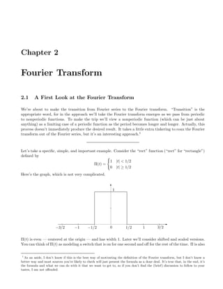
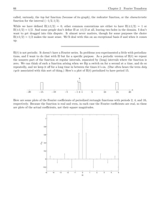
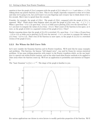
This document provides an introduction to the Fourier transform through the example of a rectangular function Π(t). It begins by discussing how to obtain the Fourier transform by taking the limit as the period of the periodic rectangular function goes to infinity. This produces the Fourier transform integral definition. It then calculates the Fourier transform of Π(t) to be the sinc function. Finally, it discusses how the inverse Fourier transform allows recovering the original function f(t) from its Fourier transform f^(s) via Fourier inversion.