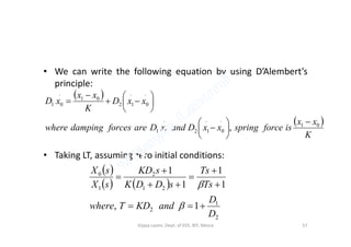
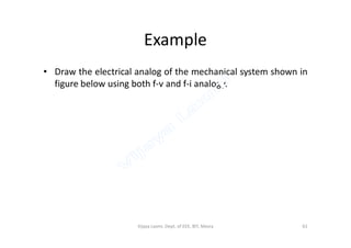
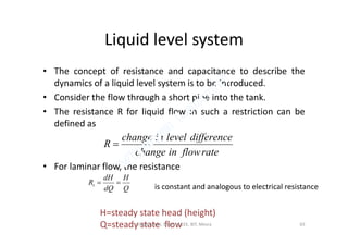
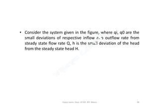
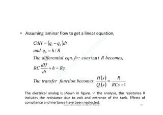
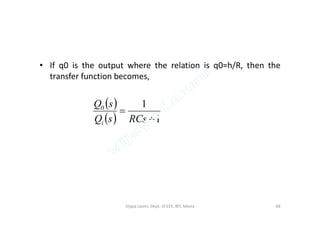
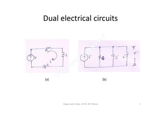
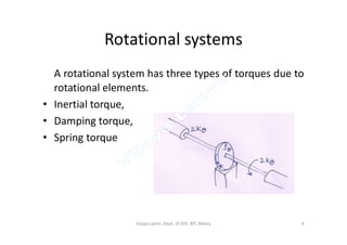
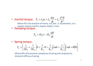
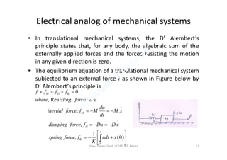
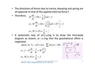
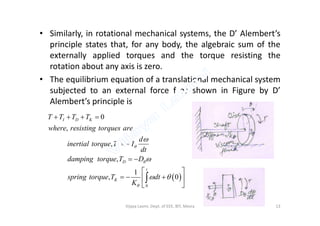
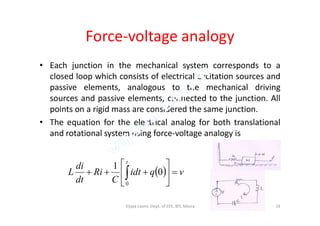
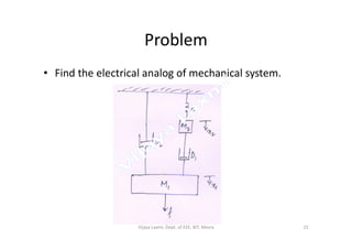
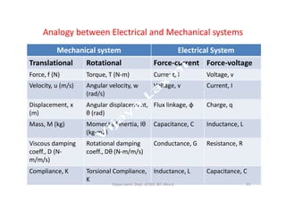
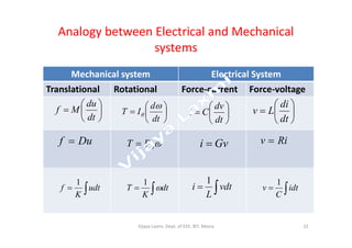
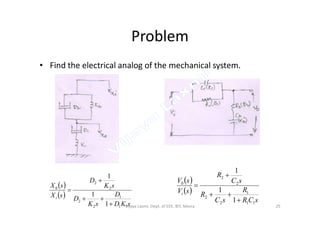
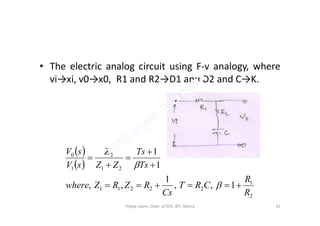
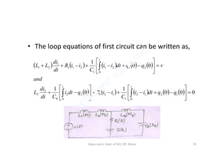
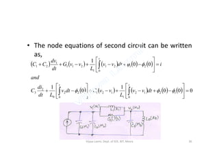
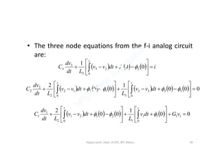
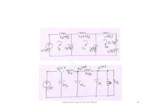
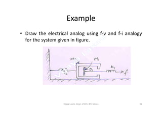
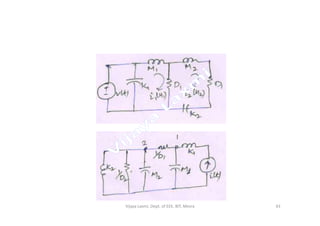
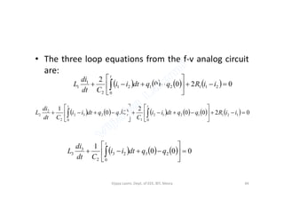
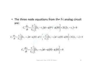
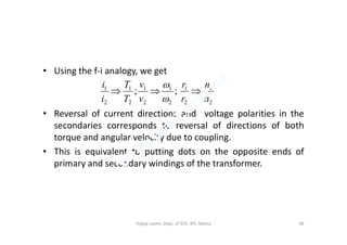
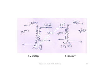
The document discusses analogous systems and provides examples of electrical-mechanical analogies. Analogous systems are physical systems that can be described by identical differential equations or transfer functions. An electrical system of resistors, capacitors and inductors may be analogous to a mechanical system of masses, dampers and springs. The equations for a translational mechanical system subjected to force are analogous to electrical circuit equations. Similarly, the equations for a rotational mechanical system subjected to torque are analogous to other electrical circuit equations. The document provides examples of modeling translational and rotational mechanical systems and their electrical analogies using either force-voltage or force-current analogies. Key components are mapped between the two domains.

1. Module II
Analogous SystemsAnalogous Systems
1Vijaya Laxmi, Dept. of EEE, BIT, Mesra

2. • For analysis of a dynamic system, derivation of
mathematical model is important.
• The mathematical model of any system, electrical,
mechanical, electro-mechanical, acoustic etc., can be
obtained provided the dynamics of the system under
investigation is known.investigation is known.
• The concept of analogous system is very useful since one
type of system may be easier to handle experimentally
than another.
• If the response of any physical system for a given
excitation is determined, the response of other systems,
which can be described by the same set of equations are
known for the same excitation function.
2Vijaya Laxmi, Dept. of EEE, BIT, Mesra

3. • Systems remain analogous as long as their differential
equations or transfer functions are of identical forms.
• A given electrical system consisting of resistances,
capacitances and inductances may be analogous to a
mechanical system consisting of a suitable combinationmechanical system consisting of a suitable combination
of dashpot, mass and spring.
• The electrical system may be analogous to any other kind
of system.
• Dual electrical systems are special kind of analogous
systems.
3Vijaya Laxmi, Dept. of EEE, BIT, Mesra

4. Dual electrical circuits
(a) (b)
4Vijaya Laxmi, Dept. of EEE, BIT, Mesra

5. • For (a), the equations are:
• For (b), the equations are:
  vqidt
C
Ri
dt
di
L
t






  0
1
0
• For (b), the equations are:
  '0'
'
1
'
'
'
0
idtv
L
Gv
dt
dv
C
t






  
The two circuits are dual where R→G, L→C’, C→L’, i→v’, v→I’
5Vijaya Laxmi, Dept. of EEE, BIT, Mesra

6. Objectives
• To provide the tools and experience to create models
of physical systems found in electrical, mechanical,
electromechanical and liquid level systems.
• To find the electrical analogy of mechanical system,To find the electrical analogy of mechanical system,
electromechanical and liquid level systems.
6Vijaya Laxmi, Dept. of EEE, BIT, Mesra

7. Translational systems
A translational system has three types of forces due
to passive elements.
• Inertial force, due to inertial mass
• Viscous damping force, due to viscous damping• Viscous damping force, due to viscous damping
• Spring force
7Vijaya Laxmi, Dept. of EEE, BIT, Mesra

8. • Inertial force:
• Viscous damping force: It is the retarding force
proportional to velocity u and given by
2
2
dt
td
M
dt
du
MMafM 
Where x is the displacement, u is velocity and a is acceleration
proportional to velocity u and given by
• Spring force:
dt
dx
DDufD 
Where D is the coefficient of damping
Where K is the compliance of spring and reciprocal to spring constant


















 
t
K xudt
K
dtu
K
x
K
f
0
)0(
111
8Vijaya Laxmi, Dept. of EEE, BIT, Mesra

9. Rotational systems
A rotational system has three types of torques due to
rotational elements.
• Inertial torque,
• Damping torque,• Damping torque,
• Spring torque
9Vijaya Laxmi, Dept. of EEE, BIT, Mesra

10. • Inertial torque:
• Damping torque:
2
2
dt
d
I
dt
d
IITI

  
Where Iθ is the moment of inertia, α is angular acceleration, w is
angular velocity and θ is angular displacement.
d
DDT

 
• Spring torque:
dt
d
DDTD

  
 











 
t
K dt
K
dt
KKKK
T
0
0
111
2
1
2
1


Where Kθ is the torsional compliance of spring and reciprocal to
torsional stiffness of spring
10Vijaya Laxmi, Dept. of EEE, BIT, Mesra

11. Electrical analog of mechanical systems
• In translational mechanical systems, the D’ Alembert’s
principle states that, for any body, the algebraic sum of the
externally applied forces and the forces resisting the motion
in any given direction is zero.
• The equilibrium equation of a translational mechanical system
subjected to an external force f as shown in Figure below bysubjected to an external force f as shown in Figure below by
D’ Alembert’s principle is
 
..
.
0
0
, Re
,
,
1
, 0
M D K
M
D
t
K
f f f f
where sisting forces are
du
inertial force f M M x
dt
damping force f Du D x
spring force f udt x
K
   
   
   
 
   
 

11Vijaya Laxmi, Dept. of EEE, BIT, Mesra

12. • The directions of forces due to inertia, damping and spring are
all opposite to that of the applied external force f.
• Therefore,
A systematic way of analyzing is to draw the free-body
 
f
K
x
xDxMor
fxudt
K
Du
dt
du
Mor
fudt
K
Du
dt
du
M
t











...
0
,
0
1
,
1
• A systematic way of analyzing is to draw the free-body
diagram as shown, assuming that the gravitational effect is
neglected.
K
f
K
x
xDxMor
dt
xd
M
K
x
dt
dx
Dfor
MaforceslawsNewtonbyAgain



...
2
2
,
,
,',
Both the equations are same. 12Vijaya Laxmi, Dept. of EEE, BIT, Mesra

13. • Similarly, in rotational mechanical systems, the D’ Alembert’s
principle states that, for any body, the algebraic sum of the
externally applied torques and the torque resisting the
rotation about any axis is zero.
• The equilibrium equation of a translational mechanical system
subjected to an external force f as shown in Figure by D’
Alembert’s principle is
0T T T T   
 
0
0
,
,
,
1
, 0
I D K
I
D
t
K
T T T T
where resisting torques are
d
inertial torque T I
dt
damping torque T D
spring torque T dt
K





 
   
 
 
 
   
 

13Vijaya Laxmi, Dept. of EEE, BIT, Mesra

14. Force-voltage analogy
• Each junction in the mechanical system corresponds to a
closed loop which consists of electrical excitation sources and
passive elements, analogous to the mechanical driving
sources and passive elements, connected to the junction. All
points on a rigid mass are considered the same junction.points on a rigid mass are considered the same junction.
• The equation for the electrical analog for both translational
and rotational system using force-voltage analogy is
  vqidt
C
Ri
dt
di
L
t






  0
1
0
14Vijaya Laxmi, Dept. of EEE, BIT, Mesra

15. Problem
• Find the electrical analog of mechanical system.
15Vijaya Laxmi, Dept. of EEE, BIT, Mesra

16. Solution
• For M1:
   211
21
1
1
12
1
2
1
1
1
uuD
dt
xxd
Df
dt
du
M
dt
xd
Mf
D
M




12
2
22
uD
dt
dx
Df
dt
D 
 
  fuDuDD
dt
du
M
fuDuuD
dt
du
M
RulesAlembertDBy


21121
1
1
12211
1
1
,''
16Vijaya Laxmi, Dept. of EEE, BIT, Mesra

17. • For M2:
   





D
M
uuD
dt
xxd
Df
dt
du
M
dt
xd
Mf
121
12
1
2
22
2
2
2
1
2
 





 
t
K xdtu
K
x
K
f
0
222 0
11
  00
1
,''
0
2221
2
211 





 
t
xdtu
K
uD
dt
du
MuD
RulesAlembertDBy
17Vijaya Laxmi, Dept. of EEE, BIT, Mesra

18.   viRiRR
dt
di
LLoop  21121
1
1:1
  00
1
:2
0
2221
2
211 





 
t
qdti
C
iR
dt
di
LiRLoop
18Vijaya Laxmi, Dept. of EEE, BIT, Mesra

19. Force-current analogy
• Each junction in the mechanical system corresponds to a node
or junction which joins electrical excitation sources and
passive elements, analogous to the mechanical driving
sources and passive elements, connected to the junction. All
points on a rigid mass are considered the same junction. One
terminal of capacitance analogous to mass is alwaysterminal of capacitance analogous to mass is always
connected to ground.
• The equation for the electrical analog for both translational
and rotational system using force-current analogy is
  '0''
'
1
'
'
'
0
idtv
L
Gv
dt
dv
C
t






  
19Vijaya Laxmi, Dept. of EEE, BIT, Mesra

20.   ivGvGG
dt
dv
CNode  21121
1
1:1
  00
1
:2
0
2221
2
211 





 
t
dtv
L
vG
dt
dv
CvGNode 
20Vijaya Laxmi, Dept. of EEE, BIT, Mesra

21. Analogy between Electrical and Mechanical systems
Mechanical system Electrical System
Translational Rotational Force-current Force-voltage
Force, f (N) Torque, T (N-m) Current, I Voltage, v
Velocity, u (m/s) Angular velocity, w
(rad/s)
Voltage, v Current, I
Displacement, x Angular displacement, Flux linkage, φ Charge, qDisplacement, x
(m)
Angular displacement,
θ (rad)
Flux linkage, φ Charge, q
Mass, M (kg) Moment of inertia, Iθ
(kg-m2)
Capacitance, C Inductance, L
Viscous damping
coeff., D (N-
m/m/s)
Rotational damping
coeff., Dθ (N-m/m/s)
Conductance, G Resistance, R
Compliance, K Torsional Compliance,
K
Inductance, L Capacitance, C
21Vijaya Laxmi, Dept. of EEE, BIT, Mesra

22. Analogy between Electrical and Mechanical
systems
Mechanical system Electrical System
Translational Rotational Force-current Force-voltage







dt
du
Mf 






dt
d
IT

 






dt
dv
Ci 






dt
di
Lv
  dt  dt
Duf  DT  Gvi  Riv 
 vdt
L
i
1
 udt
K
f
1
 dt
K
T 
1
 idt
C
v
1
22Vijaya Laxmi, Dept. of EEE, BIT, Mesra

23. Problem
• Find the electrical analog of the mechanical system.
 
  1
10


DKssX
sX
i
 
  1
10


RCssV
sV
i
23Vijaya Laxmi, Dept. of EEE, BIT, Mesra

24. Problem
• Find the electrical analog of the mechanical system.
 
  1
0


DKs
DKs
sX
sX
i
 
  1
0


RCs
RCs
sV
sV
i
24Vijaya Laxmi, Dept. of EEE, BIT, Mesra

25. Problem
• Find the electrical analog of the mechanical system.
 
 
sKD
D
sK
D
sK
D
sX
sX
i
11
1
2
2
2
2
0
1
1
1




 
 
sCR
R
sC
R
sC
R
sV
sV
i
11
1
2
2
2
2
0
1
1
1




25Vijaya Laxmi, Dept. of EEE, BIT, Mesra

26. Example
• Draw the electric analog and derive the transfer function of a
mechanical lead network as shown in figure, where x1=input
displacement, x0=output displacement, y=displacement of
the spring, D1, D2=viscous damping coefficients and
K=compliance of the spring.
26Vijaya Laxmi, Dept. of EEE, BIT, Mesra

27. • By D’ Alembert’s principle,
..
01
..
01
.
0
.
12
K
y
yxDand
yxDxxD




















• Taking LT, assuming zero initial conditions:
./
..
01
.
0
.
12
Kyisforcespringtheand
yxDandxxDareforcesdampingwhere
K














 
     
 2121
21
2
1212
1
1
0
/,,
/1
/1
1/
1
DDDKDTwhere
Ts
Ts
DD
D
sKDDDD
KsD
sX
sX











27Vijaya Laxmi, Dept. of EEE, BIT, Mesra

28. • The electric analog circuit using F-v analogy, where
vi→xi, v0→x0, R1 and R2→D1 and D2 and C→K.
 
 
   21
1
122
1
1
1
21
2
1
0
,,,
1
,
/1
/1
RR
R
CRTRZ
CsR
R
Zwhere
Ts
Ts
ZZ
Z
sV
sV











28Vijaya Laxmi, Dept. of EEE, BIT, Mesra

29. Example
• Consider the mechanical lag network shown in the
figure, where x1=input displacement, x2= output
displacement, D1, D2= viscous damping coefficients
and K=compliance.
29Vijaya Laxmi, Dept. of EEE, BIT, Mesra

30. • We can write the following equation by using D’ Alembert’s
principle:
 
 xx
isforcespringxxDandxDareforcesdampingwhere
xxD
K
xx
xD
01
...
.
0
.
12
01
.
01
,















• Taking LT, assuming zero initial conditions:
 
K
xx
isforcespringxxDandxDareforcesdampingwhere 01
01201 ,








 
   
2
1
2
21
2
1
0
1,
1
1
1
1
D
D
andKDTwhere
Ts
Ts
sDDK
sKD
sX
sX









30Vijaya Laxmi, Dept. of EEE, BIT, Mesra

31. • The electric analog circuit using F-v analogy, where
vi→xi, v0→x0, R1 and R2→D1 and D2 and C→K.
 
 
2
1
22211
21
2
1
0
1,,
1
,,
1
1
R
R
CRT
Cs
RZRZwhere
Ts
Ts
ZZ
Z
sV
sV








31Vijaya Laxmi, Dept. of EEE, BIT, Mesra

32. Example
• Draw the electrical analogous circuit of the
mechanical system given in figure below.
32Vijaya Laxmi, Dept. of EEE, BIT, Mesra

33. • The force equations of two masses are given by,
 
011
..
1
21
..
11




xx
xMand
tASin
K
xx
xM 
 
0
21
1
1
1
22 


KK
x
K
x
xMand
 
 
tASinvxiKCMLiqwhere
CC
q
C
q
qLand
v
C
qq
qL
areequationsKVLThe







,,,,,
0
,
.
21
1
1
1
..
22
1
21
..
11
33Vijaya Laxmi, Dept. of EEE, BIT, Mesra

34. Example
• Draw the electrical analog of the mechanical system shown in
figure below using both f-v and f-i analogy.
34Vijaya Laxmi, Dept. of EEE, BIT, Mesra

35. • The loop equations of first circuit can be written as,
         00
1
0
2121
1
211
1
21 





 
t
and
vqqdtii
C
iiR
dt
di
LL
          000
1
0
1
0
1212
1
121
0
22
0
2
3 











 
tt
qqdtii
C
iiRqdti
Cdt
di
L
and
35Vijaya Laxmi, Dept. of EEE, BIT, Mesra

36. • The node equations of second circuit can be written
as,
         00
1
0
2121
1
211
1
21 





 
t
and
idtvv
L
vvG
dt
dv
CC 
          000
1
0
1
0
1212
1
121
0
22
0
2
3 











 
tt
dtvv
L
vvGdtv
Ldt
di
C
and

36Vijaya Laxmi, Dept. of EEE, BIT, Mesra

37. Example
• Draw the electrical analog using f-v and f-i analogy for the
system given in figure with f=FSinwt.
37Vijaya Laxmi, Dept. of EEE, BIT, Mesra

38. • For M3:
• For M2:
      tFSinfxxdtuu
Kdt
du
M
t






  00
1
2
0
323
3
3
3
            000
1
00
22




  xxdtuuxxdtuu
du
M
tt
• For M1:
            000
1
00
2
3
0
232
3
1
0
212
2
2
2 











  xxdtuu
K
xxdtuu
Kdt
du
M
        00
1
00
2
11
0
11
1
2
0
121
2
1
1 











  uDxdtu
K
xxdtuu
Kdt
du
M
tt
The electric analog circuits are drawn
38Vijaya Laxmi, Dept. of EEE, BIT, Mesra

39. • The three node equations from the f-i analog circuit
are:
      idtvv
Ldt
dv
C
t






  00
1
2
0
323
3
3
3 
            000
1
00
2
3
0
232
3
1
0
212
2
2
2 











  
tt
dtvv
L
dtvv
Ldt
dv
C
        00
1
00
2
11
0
11
1
2
0
121
2
1
1 











  vGdtv
L
dtvv
Ldt
dv
C
tt

39Vijaya Laxmi, Dept. of EEE, BIT, Mesra

40. 40Vijaya Laxmi, Dept. of EEE, BIT, Mesra

41. Example
• Draw the electrical analog using f-v and f-i analogy
for the system given in figure.
41Vijaya Laxmi, Dept. of EEE, BIT, Mesra

42. • For M1:
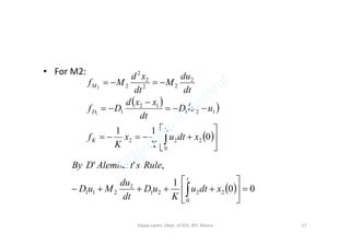
• For M2:
              0200
2
00
12








  uuDxxdtuuxxdtuu
du
M
tt
        0200
2
2112
0
121
2
1
1 





  uuDxxdtuu
Kdt
du
M
t
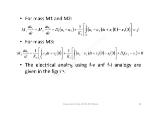
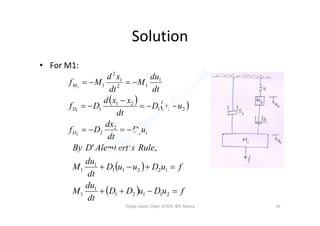
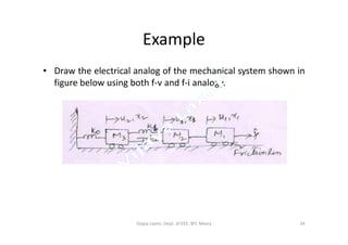
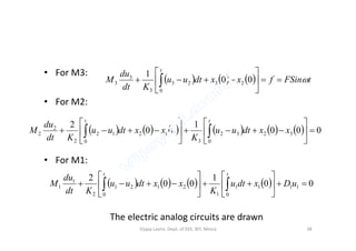
Force applied on M1 is zero, i.e., in f-v analog circuit, the first mesh
is shorted, v[f]=0. Only the mesh current i1[u1] is flowing in mesh 1.
• For M3:
      000
1
0
2323
2
3
3 





 
t
xxdtuu
Kdt
du
M
              020000 1211
0
212
1
3
0
232
2
2
2 







  uuDxxdtuu
K
xxdtuu
Kdt
M
The electric analog circuits are drawn
42Vijaya Laxmi, Dept. of EEE, BIT, Mesra

43. 43Vijaya Laxmi, Dept. of EEE, BIT, Mesra

44. • The three loop equations from the f-v analog circuit
are:
        0200
2
2112
0
121
2
1
1 





  iiRqqdtii
Cdt
di
L
t
              0200
2
00
1
1211
0
212
1
3
0
232
2
2
2 











  iiRqqdtii
C
qqdtii
Cdt
di
L
tt
      000
1
2
0
323
2
3
3 





  qqdtii
Cdt
di
L
t
44Vijaya Laxmi, Dept. of EEE, BIT, Mesra

45. • The three node equations from the f-i analog circuit
are:
        0200
2
2112
0
121
2
1
1 





  vvGdtvv
Ldt
dv
C
t

              0200
2
00
1
1211
0
212
1
3
0
232
2
2
2 











  vvGdtvv
L
dtvv
Ldt
dv
C
tt

      000
1
2
0
323
2
3
3 





  
t
dtvv
Ldt
dv
C
45Vijaya Laxmi, Dept. of EEE, BIT, Mesra

46. Mechanical couplings
• Common mechanical coupling devices, i.e., friction wheels,
gear trains, levers, etc. also have electrical analogs.
• These mechanical coupling deices act as matching devices like
transformers in electrical systems.
• These mechanical devices transmit energy from one part of a• These mechanical devices transmit energy from one part of a
system to another in such a way that force, torque, speed and
displacement are altered.
• The inertia and friction of these mechanical coupling devices
are neglected in the ideal case considered.
• The relationships between torques, angular displacements,
angular velocities, radii and number of teeth of the
mechanical coupling devices are derived as follows:
46Vijaya Laxmi, Dept. of EEE, BIT, Mesra

47. Friction wheels
• The points of contact on wheel 1 and 2 must have the same
linear velocity because they move together and experience
equal and opposite forces. Being a rotational system, it is
convenient to use angular velocity and torques. So,
rrT 
• The electrical analog of the friction wheel-pair is an ideal
transformer having the turns ratio n1:n2.
• The f-v analogy can be written as
2
1
2
1
2
1
2
1
r
r
and
r
r
T
T



2
1
2
1
2
1
2
1
2
1
2
1
;;
T
T
v
v
n
n
r
r
i
i



47Vijaya Laxmi, Dept. of EEE, BIT, Mesra

48. • Using the f-i analogy, we get
• Reversal of current directions and voltage polarities in the
secondaries corresponds to reversal of directions of both
2
1
2
1
2
1
2
1
2
1
2
1
;;
n
n
r
r
v
v
T
T
i
i



secondaries corresponds to reversal of directions of both
torque and angular velocity due to coupling.
• This is equivalent to putting dots on the opposite ends of
primary and secondary windings of the transformer.
48Vijaya Laxmi, Dept. of EEE, BIT, Mesra

49. F-V analogy F-i analogy
49Vijaya Laxmi, Dept. of EEE, BIT, Mesra

50. Gear trains
• These are used in control systems to attain mechanical matching of
motor to load.
• Generally, servomotor operates at a high speed but has low torque.
To drive a load with high torque and low speed by such a motor,
speed reduction and torque magnification are achieved by gear
trains.
• The number of teeth on the surface of the gears is proportional to
radii r1 and r2 of the gears, i.e.,
nrnr radii r1 and r2 of the gears, i.e.,
• The distance travelled along the surface of each gear is the same.
Therefore,
• The workdone by one gear is equal to that done by the other since
there is assumed to be no loss.
2211 nrnr 
2211  rr 
2211  TT 
50Vijaya Laxmi, Dept. of EEE, BIT, Mesra

51. Mechanical lever
• Consider the mechanical system (lever) shown in the figure,
where f1 is the input force applied at the left-hand mass M1
causing a displacement x1. The equation of motion can be
written as,
'1
.
11
..
111 fxDxMf 
Where f1’ is the force acting at the hinge point 1 of the lever.Where f1’ is the force acting at the hinge point 1 of the lever.
This results in a force f2’ acting in the upward direction at hinge
point 2. Then,
nr
r
x
x
x
x
x
x
and
sayn
r
r
f
f
1
,
)(
2
1
..
2
..
1
.
2
.
1
2
1
1
2
'
2
'
1


Where n is the arms ratio
51Vijaya Laxmi, Dept. of EEE, BIT, Mesra

52. • We may also write for M1,
][, 12
2
1
1
.
2
..
12
2
2
2
2
.
2
..
22
'
2
'
2
2
2
2
.
2
..
22
'
2
nxxas
K
x
xDxMn
K
x
xDxMnnffNow
K
x
xDxMf














22 KK 
      12
2
..
12
2
1
..
12
2
11 /
,
xMnxDnDxMnMf
equationfirstinPutting

52Vijaya Laxmi, Dept. of EEE, BIT, Mesra

53. Example
• Draw the electric analog and derive the transfer
function of a mechanical lead network as shown in
figure, where x1=input displacement, x0=output
displacement, y=displacement of the spring, D1,
D2=viscous damping coefficients and K=complianceD2=viscous damping coefficients and K=compliance
of the spring.
53Vijaya Laxmi, Dept. of EEE, BIT, Mesra

54. • By D’ Alembert’s principle,
..
01
..
01
.
0
.
12
K
y
yxDand
yxDxxD




















• Taking LT, assuming zero initial conditions:
./
..
01
.
0
.
12
Kyisforcespringtheand
yxDandxxDareforcesdampingwhere
K














 
     
 2121
21
2
1212
1
1
0
/,,
/1
/1
1/
1
DDDKDTwhere
Ts
Ts
DD
D
sKDDDD
KsD
sX
sX











54Vijaya Laxmi, Dept. of EEE, BIT, Mesra

55. • The electric analog circuit using F-v analogy, where
vi→xi, v0→x0, R1 and R2→D1 and D2 and C→K.
 
 
   21
1
122
1
1
1
21
2
1
0
,,,
1
,
/1
/1
RR
R
CRTRZ
CsR
R
Zwhere
Ts
Ts
ZZ
Z
sV
sV











55Vijaya Laxmi, Dept. of EEE, BIT, Mesra

56. Example
• Consider the mechanical lag network shown in the
figure, where x1=input displacement, x2= output
displacement, D1, D2= viscous damping coefficients
and K=compliance.
56Vijaya Laxmi, Dept. of EEE, BIT, Mesra

57. • We can write the following equation by using D’Alembert’s
principle:
 
 xx
isforcespringxxDandxDareforcesdampingwhere
xxD
K
xx
xD
01
...
.
0
.
12
01
.
01
,















• Taking LT, assuming zero initial conditions:
 
K
xx
isforcespringxxDandxDareforcesdampingwhere 01
01201 ,








 
   
2
1
2
21
2
1
0
1,
1
1
1
1
D
D
andKDTwhere
Ts
Ts
sDDK
sKD
sX
sX









57Vijaya Laxmi, Dept. of EEE, BIT, Mesra

58. • The electric analog circuit using F-v analogy, where
vi→xi, v0→x0, R1 and R2→D1 and D2 and C→K.
 
 
2
1
22211
21
2
1
0
1,,
1
,,
1
1
R
R
CRT
Cs
RZRZwhere
Ts
Ts
ZZ
Z
sV
sV








58Vijaya Laxmi, Dept. of EEE, BIT, Mesra

59. Example
• Draw the electrical analogous circuit of the
mechanical system given in figure below.
59Vijaya Laxmi, Dept. of EEE, BIT, Mesra

60. • The force equations of two masses are given by,
 
011
..
1
21
..
11




xx
xMand
tASin
K
xx
xM 
 
0
21
1
1
1
22 


KK
x
K
x
xMand
 
 
tASinvxiKCMLiqwhere
CC
q
C
q
qLand
v
C
qq
qL
areequationsKVLThe







,,,,,
0
,
.
21
1
1
1
..
22
1
21
..
11
60Vijaya Laxmi, Dept. of EEE, BIT, Mesra

61. Example
• Draw the electrical analog of the mechanical system shown in
figure below using both f-v and f-i analogy.
61Vijaya Laxmi, Dept. of EEE, BIT, Mesra

62. • For mass M1 and M2:
• For mass M3:
        fxxdtuu
K
uuD
dt
du
M
dt
du
M
t






 0
2121
1
211
1
2
1
1 00
1
          000
1
0
1
121
0
1212
10
22
0
2
3 











  uuDxxdtuu
K
xdtu
Kdt
du
M
tt
• The electrical analog using f-v anf f-i analogy are
given in the figure.
0100 
 KKdt
62Vijaya Laxmi, Dept. of EEE, BIT, Mesra

63. • The loop equations of first circuit can be written as,
         00
1
0
2121
1
211
1
21 





 
t
and
vqqdtii
C
iiR
dt
di
LL
          000
1
0
1
0
1212
1
121
0
22
0
2
3 











 
tt
qqdtii
C
iiRqdti
Cdt
di
L
and
63Vijaya Laxmi, Dept. of EEE, BIT, Mesra

64. • The node equations of second circuit can be written
as,
         00
1
0
2121
1
211
1
21 





 
t
and
idtvv
L
vvG
dt
dv
CC 
          000
1
0
1
0
1212
1
121
0
22
0
2
3 











 
tt
dtvv
L
vvGdtv
Ldt
di
C
and

64Vijaya Laxmi, Dept. of EEE, BIT, Mesra

65. Liquid level system
• The concept of resistance and capacitance to describe the
dynamics of a liquid level system is to be introduced.
• Consider the flow through a short pipe into the tank.
• The resistance R for liquid flow in such a restriction can be
defined asdefined as
• For laminar flow, the resistance
rateflowinchange
differencelevelinchange
R 
Q
H
dQ
dH
Rt 
is constant and analogous to electrical resistance
H=steady state head (height)
Q=steady state flow 65Vijaya Laxmi, Dept. of EEE, BIT, Mesra

66. • Consider the system given in the figure, where qi, q0 are the
small deviations of respective inflow and outflow rate from
steady state flow rate Q, h is the small deviation of the head
from the steady state head H.
66Vijaya Laxmi, Dept. of EEE, BIT, Mesra

67. • Assuming laminar flow to get a linear equation,
 
,tan.
/0
0


becomesRtconsforeqnaldifferentiThe
Rhqand
dtqqCdH i
 
  1
,
,tan.



RCs
R
sQ
sH
becomesfunctiontransferThe
Rqh
dt
dH
RC
becomesRtconsforeqnaldifferentiThe
i
i
The electrical analog is shown in figure. In the analysis, the resistance R
includes the resistance due to exit and entrance of the tank. Effects of
compliance and inertance have been neglected.
67Vijaya Laxmi, Dept. of EEE, BIT, Mesra

68. • If q0 is the output where the relation is q0=h/R, then the
transfer function becomes,
 
  1
10


RCssQ
sQ
  1

RCssQi
68Vijaya Laxmi, Dept. of EEE, BIT, Mesra

69. Liquid level system with interactions
• Consider a liquid level system with interactions as shown in
figure.
21
2
22
2
2
1
1
1121
,
,
qq
dt
dh
Cq
R
h
qq
dt
dh
Cqhh


• Considering q1 and q2 as the respective input and output, we
get the transfer function as
2
 
    1
1
122211
2
21211
2


sCRCRCRsCCRRsQ
sQ
The electrical analog is shown in figure. In the analysis, the resistance R1
includes the resistance due to exit from tank 1 and entrance to the tank 2
and R2 is the resistance of exit of tank 2. Effects of compliance and
inertance have been neglected. 69Vijaya Laxmi, Dept. of EEE, BIT, Mesra

70. Thermal system
70Vijaya Laxmi, Dept. of EEE, BIT, Mesra