![ In order to better prepare the analysis, we must first understand the data we are working with.
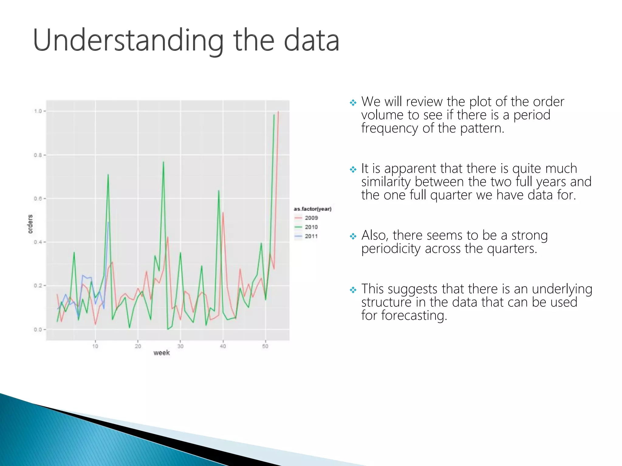
We will work on the weekly aggregates of the worldwide amount of orders, normalized into the
[0,1] interval.
The value of the week and quarter columns is relative with respect to the year. The dataset
contains values from Q1 2009 through Q1 2011.](https://image.slidesharecdn.com/16-150701043039-lva1-app6892/75/Data-Science-Part-XVI-Fourier-Analysis-25-2048.jpg)
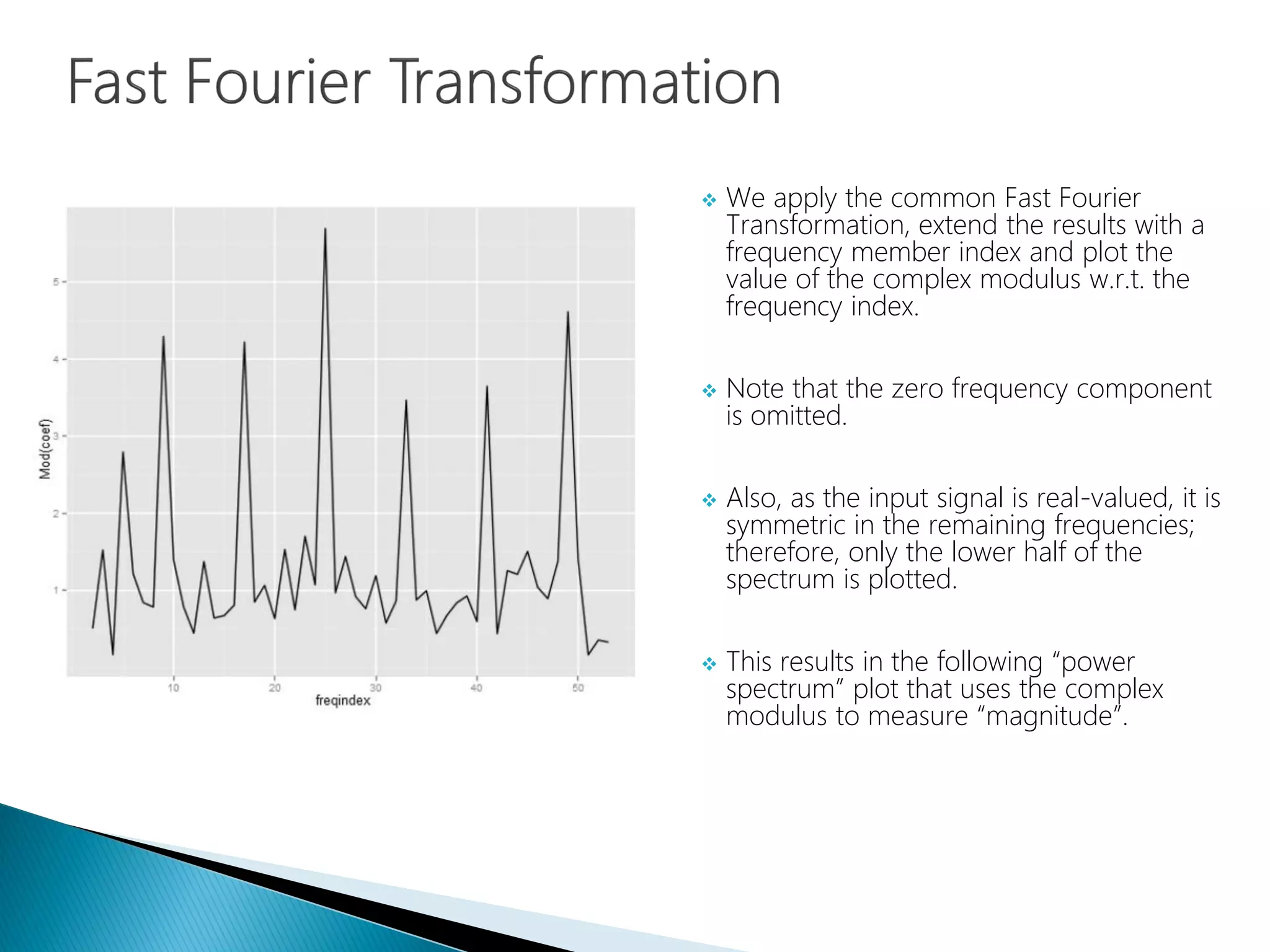


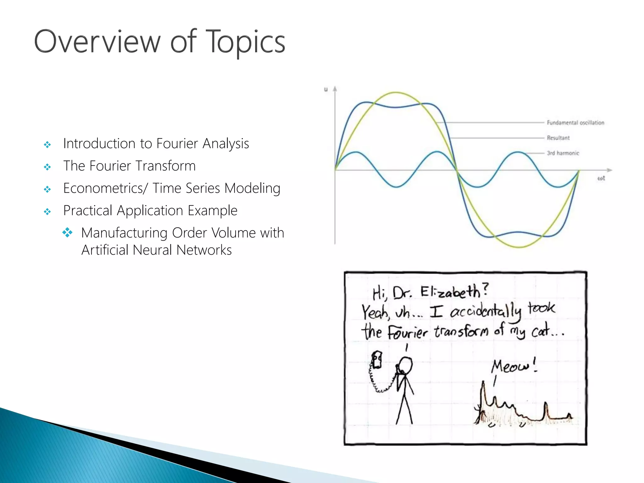
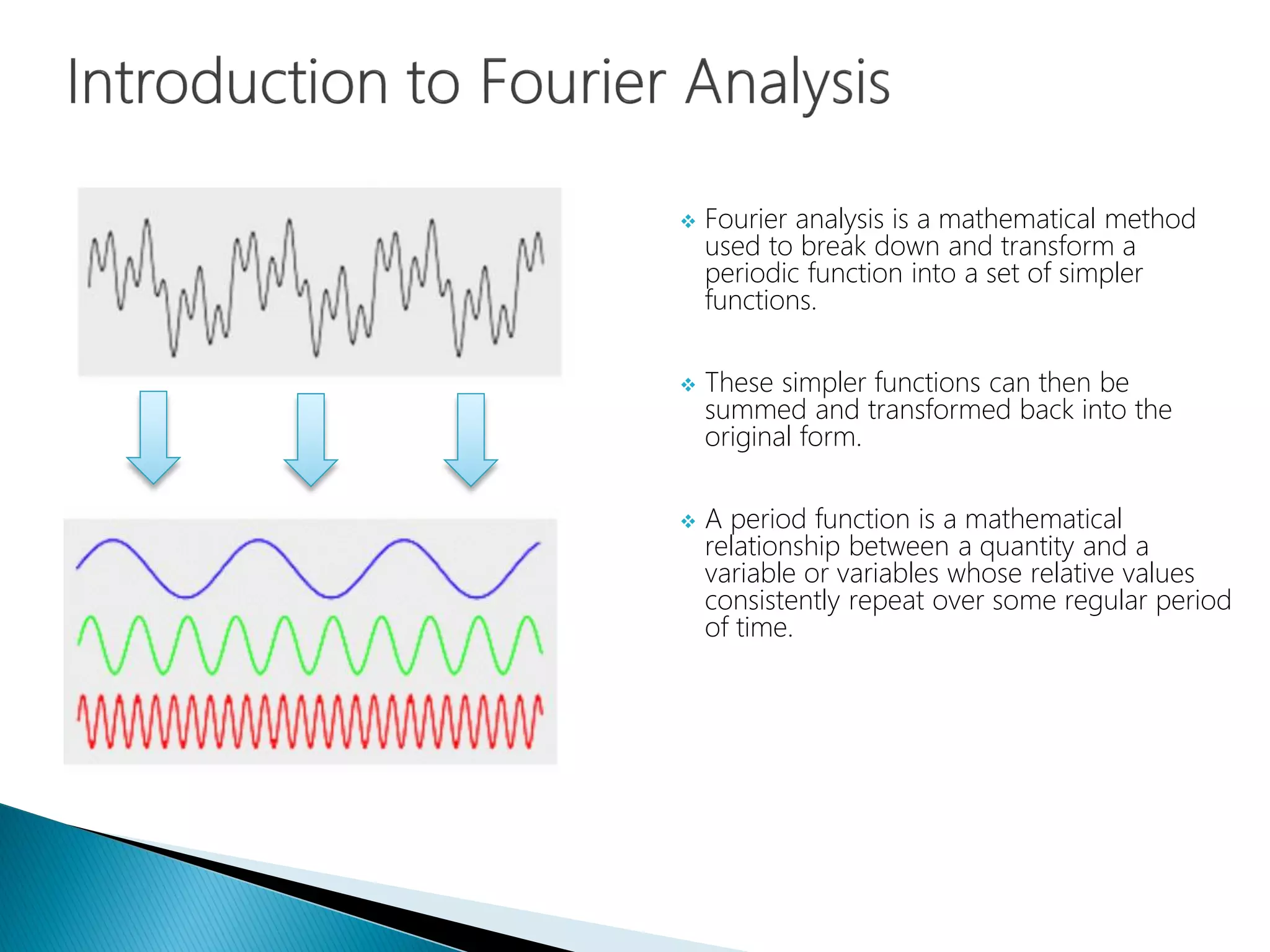
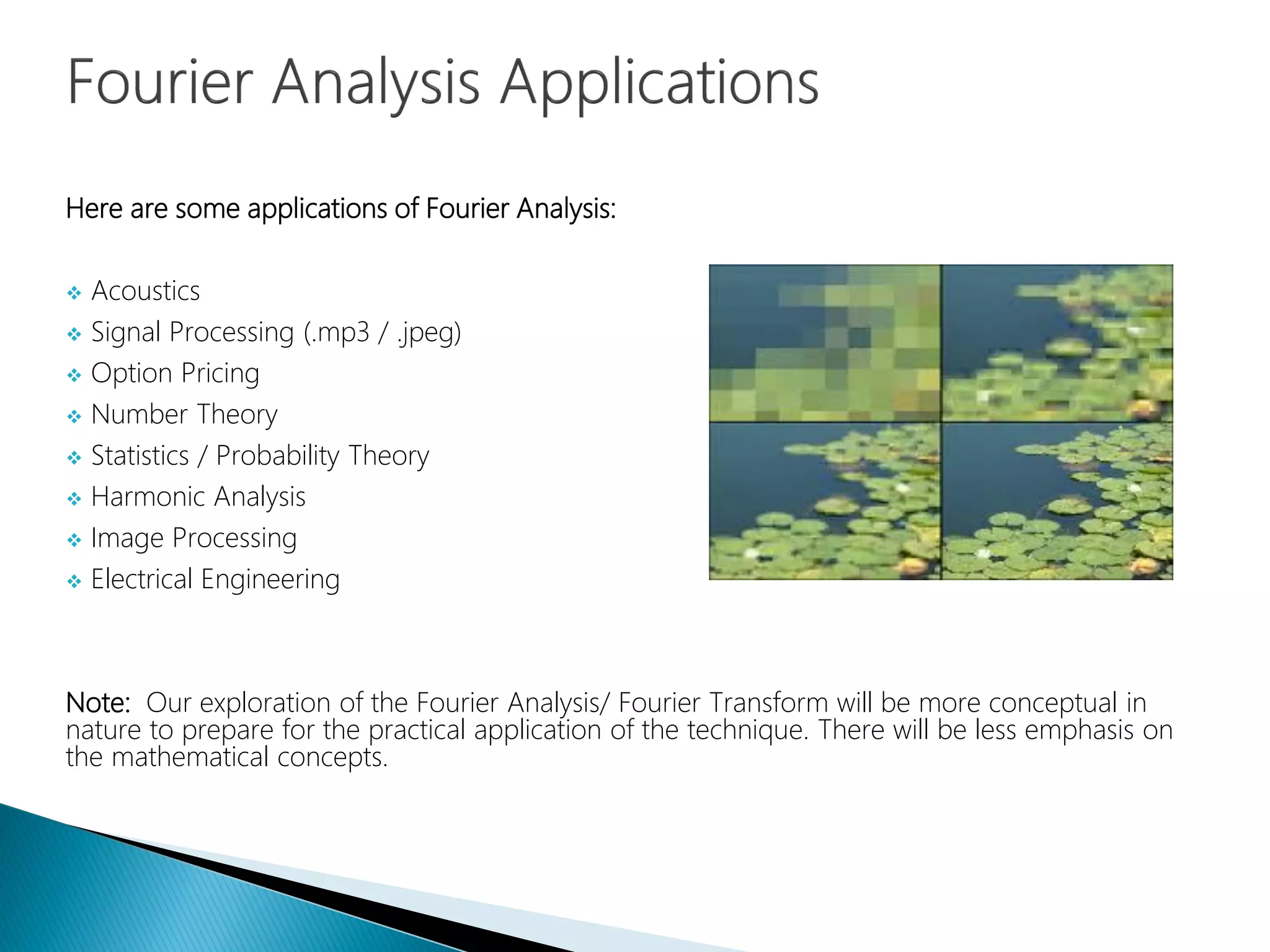
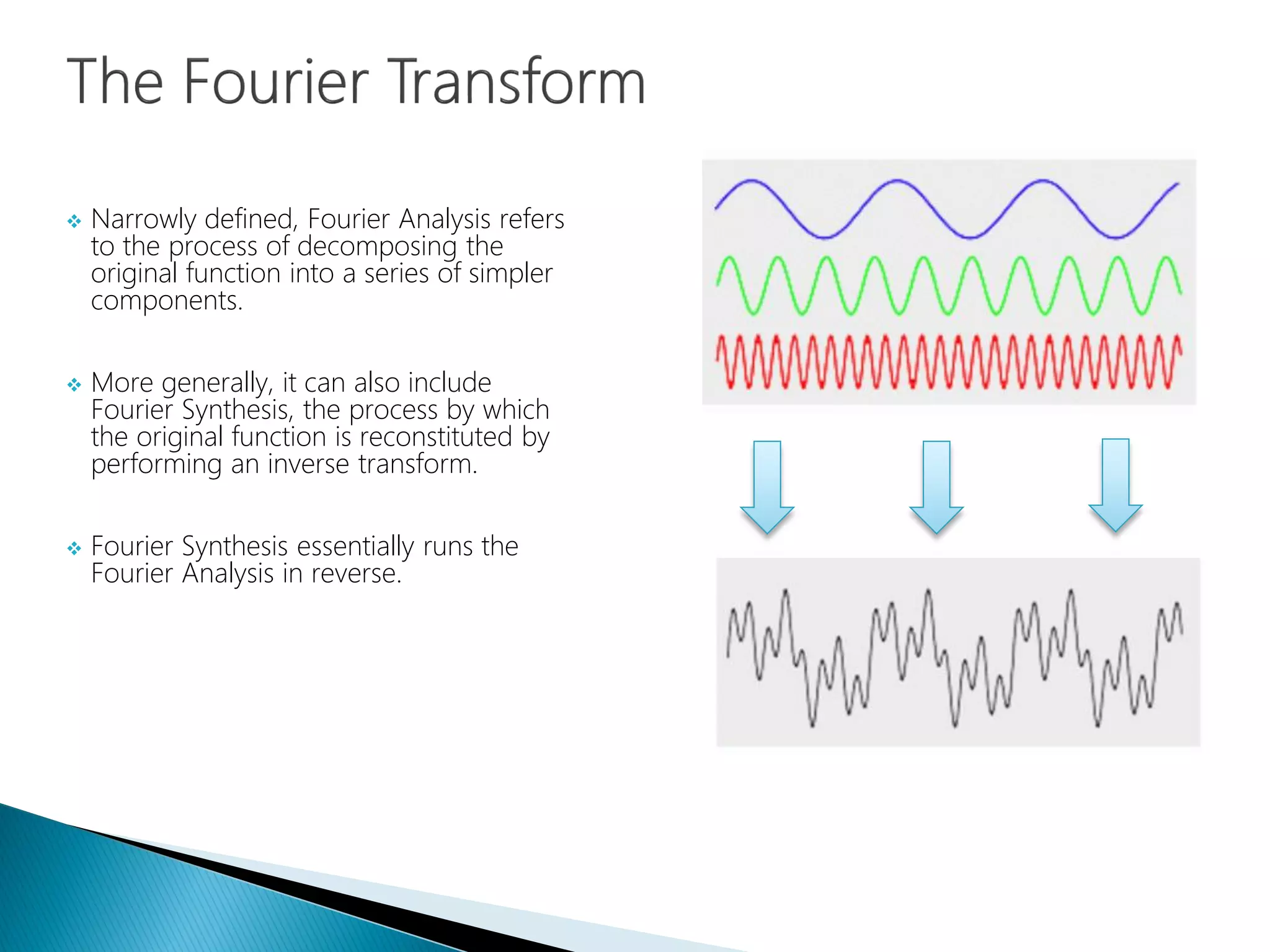
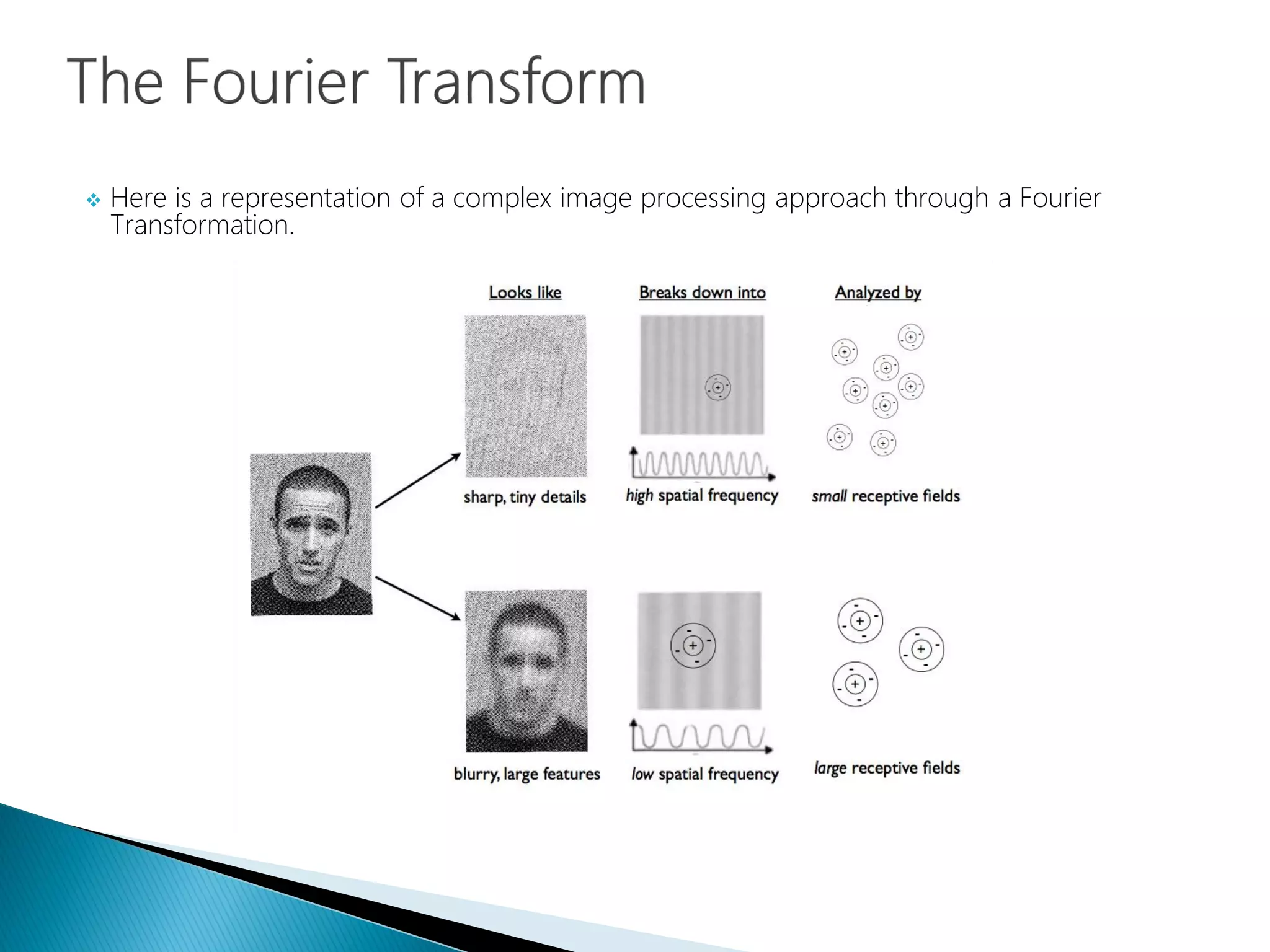
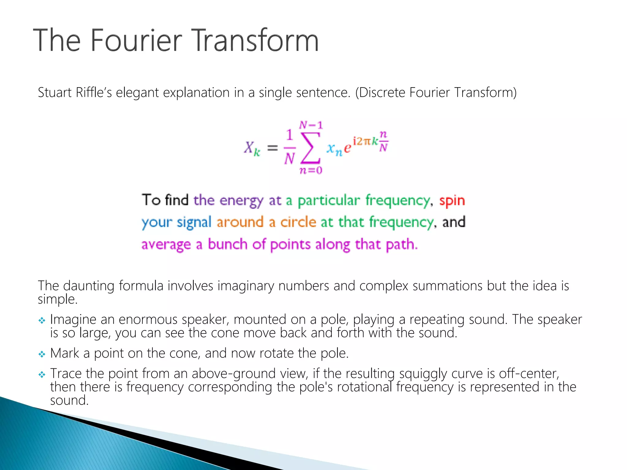
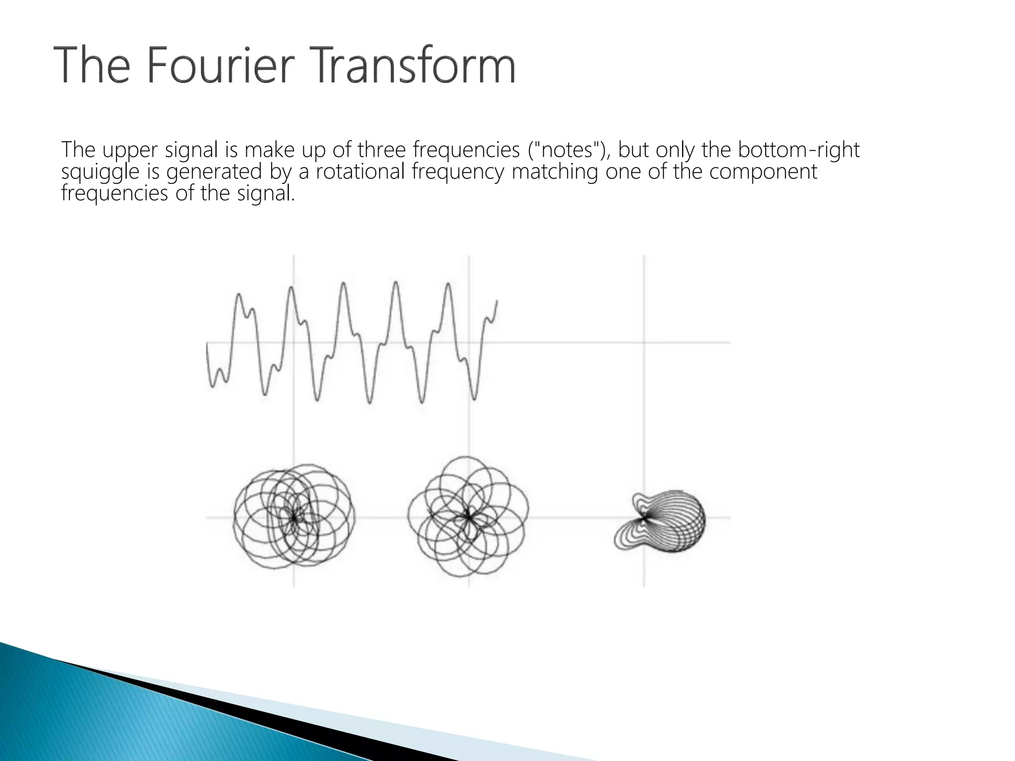
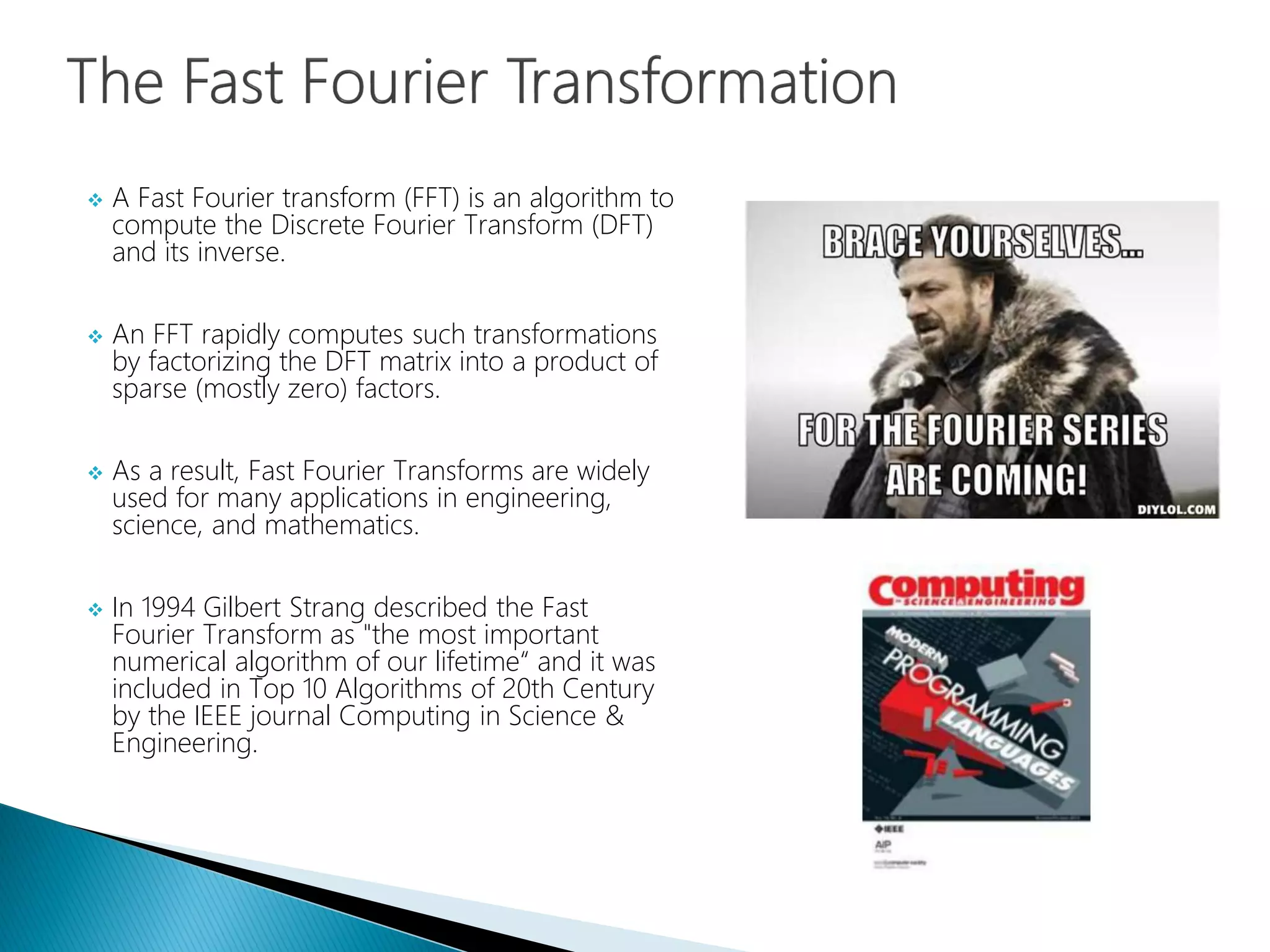
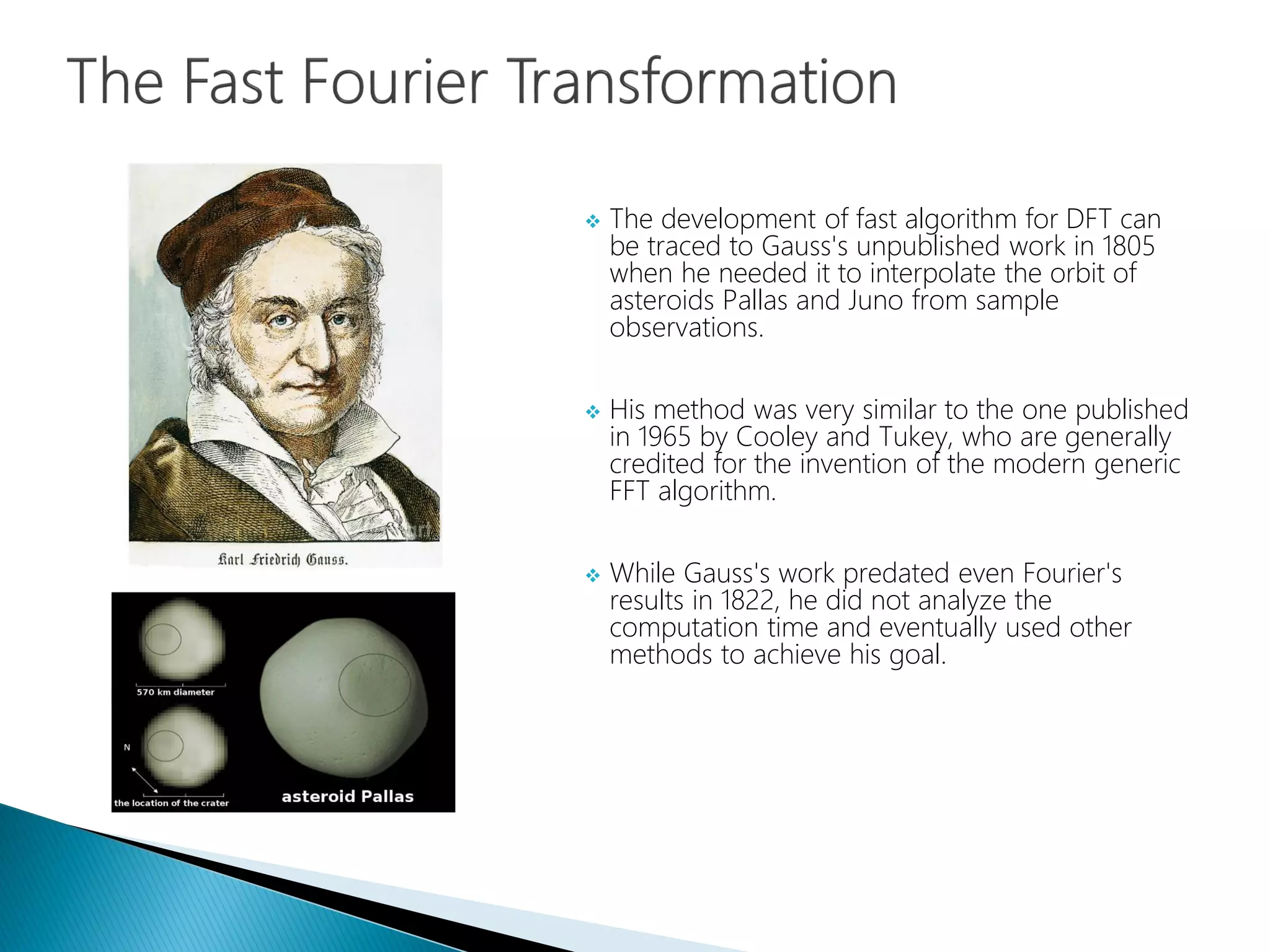
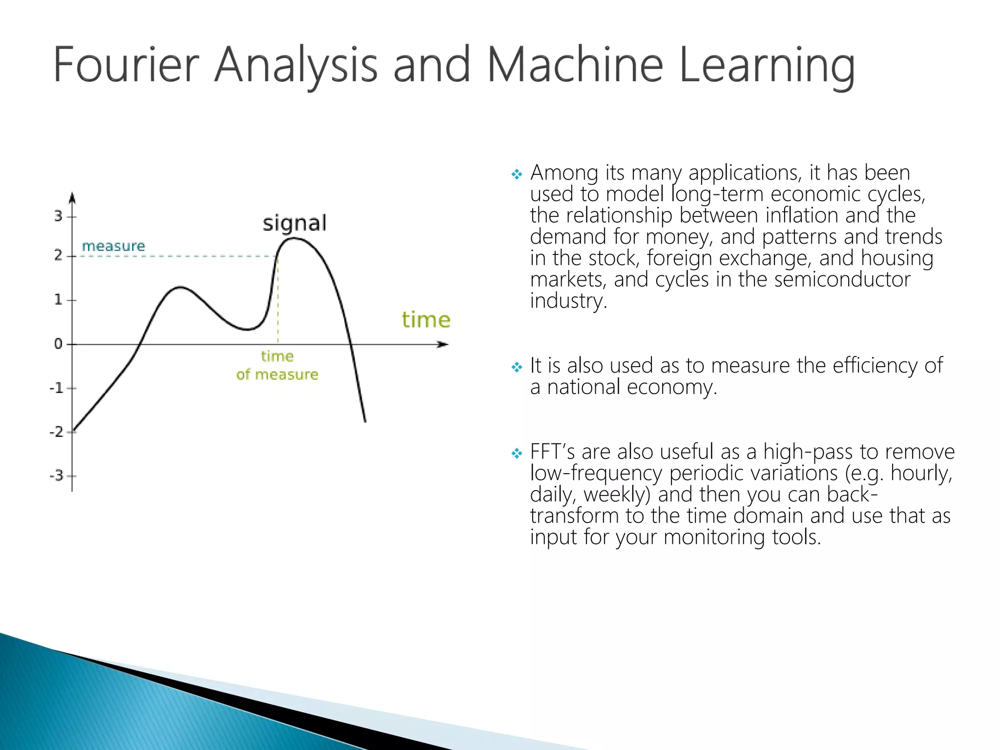
The document provides an introduction to Fourier analysis and its practical applications in forecasting manufacturing order volume using artificial neural networks. It explains the Fourier transform's role in transforming periodic functions into simpler components for analysis and synthesis, emphasizing its significance in various fields like signal processing and econometrics. Additionally, it outlines a specific approach to time series prediction by leveraging Fast Fourier Transforms (FFT) and neural networks to accurately forecast order patterns.


![[AIoTLab]attention mechanism.pptx](https://cdn.slidesharecdn.com/ss_thumbnails/aiotlabattentionmechanism-230406114603-e5ba0365-thumbnail.jpg?width=640&height=640&fit=bounds)


![[DSC Europe 25] Sara Polak - The Archaeology of Innovation: AI as the Next Cr...](https://cdn.slidesharecdn.com/ss_thumbnails/7ecbscdnt8mlcuqbd2ln-2-sara-polak-ai-creative-industries-251208152533-aa1fcf54-thumbnail.jpg?width=640&height=640&fit=bounds)


![[DSC Europe 25] Dobrica Cosic - Savings by the Second: How Dynamic Pricing an...](https://cdn.slidesharecdn.com/ss_thumbnails/znp09f3smtqz3w2sq6wn-1-dobrica-cosic-savings-by-the-second-how-dynamic-pricing-and-smart-data-are-bu-251208151905-26e6f41e-thumbnail.jpg?width=640&height=640&fit=bounds)

![[DSC Europe 25] Dunja Adzic Jovanovic - AI and Cybersecurity: Defending Data ...](https://cdn.slidesharecdn.com/ss_thumbnails/o1zylpbhrtwnixxq2xj8-7-251211083048-185086f6-thumbnail.jpg?width=640&height=640&fit=bounds)


![[DSC Europe 25] Branko Dzakula - From Defense to Attack: How AI Redefines Cyb...](https://cdn.slidesharecdn.com/ss_thumbnails/80bdzdxpr3ky2g0qvyk9-8-251211083048-ce5fc1ee-thumbnail.jpg?width=640&height=640&fit=bounds)
![[DSC Europe 25] Katherine Forrest - AI NOW: Understanding the Velocity of Cha...](https://cdn.slidesharecdn.com/ss_thumbnails/wvvbruqfrci0sfq9xwgb-4-251212104007-e5ad1987-thumbnail.jpg?width=640&height=640&fit=bounds)
![[DSC Europe 25] Dragana Ilic - AI for Big Data in Astronomy.pptx](https://cdn.slidesharecdn.com/ss_thumbnails/8palya86qaatvjhva1ms-2-dragana-ilic-ai-ilic-251208151906-652b819c-thumbnail.jpg?width=640&height=640&fit=bounds)
![[DSC Europe 25] Milan Sekuloski - Data, Defence, and Development: Cybersecuri...](https://cdn.slidesharecdn.com/ss_thumbnails/dfrkwwx4qly6atqpbl4z-4-251209104645-c3d4b0ca-thumbnail.jpg?width=640&height=640&fit=bounds)