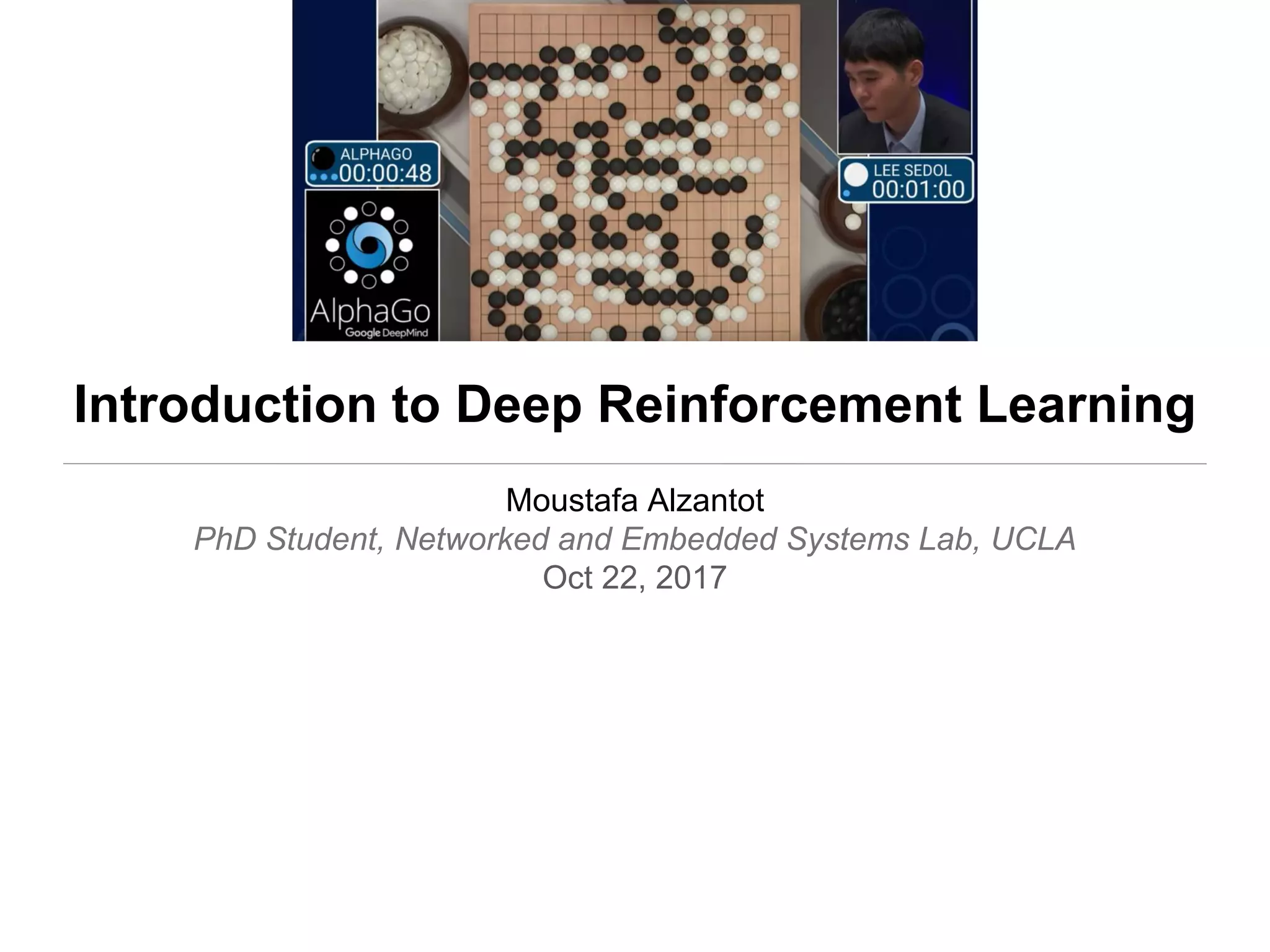
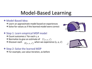
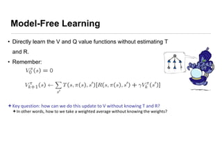
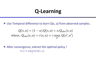
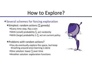
This document presents an introduction to deep reinforcement learning, outlining its foundational concepts, types, and mechanisms. It explains how agents interact with their environment to maximize rewards through various methods, including model-based and model-free learning techniques like Q-learning. The document also discusses the challenges of approximating Q-values in complex environments and introduces deep Q-networks as a solution.

1. Introduction to Deep Reinforcement Learning
Moustafa Alzantot
PhD Student, Networked and Embedded Systems Lab, UCLA
Oct 22, 2017

2. Machine Learning
Computer programs can increase their performance on a given task
without being explicitly programmed for it, just by analyzing data !

3. Types Machine Learning
• Supervised Learning
• Given a set of labeled examples , predict the output label for new unseen
inputs.
• Unsupervised Learning
• Given unlabeled dataset, understand the structure of the data (e.g.
clustering, dimensionality reduction).
• Reinforcement Learning
• Branch of machine learning concerned with acting optimally in face of
uncertainty (i.e. learning to do ! )

4. Reinforcement Learning
• Agent observes the environment state, performs some action.
• In response, the environment state changes and agent receives reward.
• Goal of agent is to pick actions that maximizes the total reward received from
environment.
Environment
Agent
Actions: a
State: s
Reward: r
Source: Pieter Abeel, UC Berkley188

5. Examples

6. Ex: Grid World
 A maze-like problem
 The agent lives in a grid
 Walls block the agent’s path
 Noisy movement: actions do not always go as planned
 80% of the time, the action North takes the agent North
(if there is no wall there)
 10% of the time, North takes the agent West; 10% East
 If there is a wall in the direction the agent would have been taken, the agent stays put
 The agent receives rewards each time step
 Small “living” reward each step (can be negative)
 Big rewards come at the end (good or bad)
 Goal: maximize sum of rewards
Source: Pieter Abeel, UC Berkley188

7. Ex: Grid World
Deterministic Grid World Stochastic Grid World

8. Markov Decision Process
• MDP is used to describe RL environments.
• MDP is defined by:
• A set of states s S
A set of actions a A
A transition function
Probability that a from s leads to s’, i.e., P(s’| s, a)
Also called the model or the dynamics
A reward function
Sometimes just R(s) or R(s’)
Discount factor
Environment
Agent
Actions: a
State: s
Reward: r
Source: Pieter Abeel, UC Berkley188

9. Discounting
It’s reasonable to maximize the sum of rewards
It’s also reasonable to prefer rewards now to rewards later
One solution: values of rewards decay exponentially
0 < < 1
Worth Now Worth Next Step Worth In Two Steps
Why discount ?
— sooner rewards will probably have higher utility than later rewards
— Control preferences of different solutions.
— Avoid numerical issues (total rewards going to infinity)

10. Optimal policy
No penalty at each step • Reward for each step: -0.1
• Reward for each step: -2 • Reward for each step: +0.1

11. Remember MDPs
• MDP is defined by:
• A set of states s S
A set of actions a A
A transition function
Probability that a from s leads to s’, i.e., P(s’| s, a)
Also called the model or the dynamics
A reward function
Sometimes just R(s) or R(s’)
Discount factor
Environment
Agent
Actions: a
State: s
Reward: r

12. Solving MDPs
• If the MDP (environment model) is known, there are ways that are guaranteed
to find the optimal policy.

13. Value-function
The value (utility) of a state s:
V*(s) = expected utility starting in s and acting optimally
The value (utility) of a q-state (s,a):
Q*(s,a) = expected utility starting out having taken action a from state s and
(thereafter) acting optimally
The optimal policy:
*(s) = optimal action from state s

14. GridWorld: Q-Values
Noise = 0.2
Discount = 0.9
Living reward = 0
Source: Pieter Abeel, UC Berkley188

15. Value Iteration
 Theorem: will converge to unique optimal values
 Basic idea: approximations get refined towards optimal values
 Policy may converge long before values do
• Alpaydin: Introduction to Machine Learning, 3rd edition

16. Policy Iteration
• Value-iterations iterates to refine the value function estimates until it
converges.
• Optimal policy often converges before the value function.
• The final goal is to get an optimal policy.
• Policy-iteration: iterates to re-define the policy at each step.
• Alpaydin: Introduction to Machine Learning, 3rd edition

17. Reinforcement Learning ?!

18. Model-Based Learning
Model-Based Idea:
Learn an approximate model based on experiences
Solve for values as if the learned model were correct
Step 1: Learn empirical MDP model
Count outcomes s’ for each s, a
Normalize to give an estimate of
Discover each when we experience (s, a, s’)
Step 2: Solve the learned MDP
For example, use value iteration, as before

19. Model-Free Learning
• Directly learn the V and Q value functions without estimating T
and R.
• Remember:
Key question: how can we do this update to V without knowing T and R?
In other words, how to we take a weighted average without knowing the weights?

20. Q-Learning
 Use Temporal difference to learn Q(s, a) from observed samples.
 After convergence, extract the optimal policy !

21. How to Explore?
Several schemes for forcing exploration
Simplest: random actions (-greedy)
Every time step, flip a coin
With (small) probability , act randomly
With (large) probability 1-, act on current policy
Problems with random actions?
You do eventually explore the space, but keep
thrashing around once learning is done
One solution: lower over time
Another solution: exploration functions

22. Demo: MountainCar using Q-Learning
https://www.youtube.com/watch?v=ByOdncJE5bE

23. Approximate Q Learning

24. Approximate Q Learning
 Basic Q-Learning keeps a table of all q-values
 In realistic situations, we cannot possibly learn about every single state!
 Too many states to visit them all in training
 Too many states to hold the q-tables in memory

25. Approximate Q-Learning
 Using a feature representation, we can write a q function (or value function) for any
state using a few weights:
 Use optimization to find the weights that minimize MSE between predicted and
observed Q-values.
Questions:
How to approximate the Q(s, a) function ?
How to compute these features ?

26. Deep Q Networks
Remember:
Universal approximation theorem:
Neural Network with 1 hidden layer can learn any
bounded continuous function!

27. Deep Q Networks
Remember:
Deep neural networks are good as feature
extractors !

28. Deep Q Networks

29. Deep Q-Network: Atari

30. Deep Q-Network training

31. Deep Q-Network training
Experience Replay Trick

32. DQN Results in Atari

33. Resources
• Pieter Abeel, UC Berkley CS 188
• Alpaydin: Introduction to Machine Learning, 3rd edition
• David Silver, UCL Reinforcement Learning Course
• Yandex: Practical RL
• MIT: Deep Learning for self-driving cars !
• Stanford 234: Reinforcement Learning

34. Thanks
Send any question to
malzantot@ucla.edu