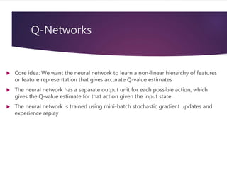
This document provides an overview of reinforcement learning and some key algorithms used in artificial intelligence. It introduces reinforcement learning concepts like Markov decision processes, value functions, temporal difference learning methods like Q-learning and SARSA, and policy gradient methods. It also describes deep reinforcement learning techniques like deep Q-networks that combine reinforcement learning with deep neural networks. Deep Q-networks use experience replay and fixed length state representations to allow deep neural networks to approximate the Q-function and learn successful policies from high dimensional input like images.

1. Reinforcement Learning in Artificial
intelligence
PRESENTED BY
S.VIJAYALAKSHMI I- MSC (IT)
Nadar Saraswathi College of
arts and science, Theni
Department of CS &IT

2. Reinforcement learning

3. Overview
 Introduction to Reinforcement Learning
 Finite Markov Decision Processes
 Temporal-Difference Learning (SARSA, Q-learning, Deep Q-Networks)
 Policy Gradient Methods (Finite Difference Policy Gradient, REINFORCE, Actor-
Critic)
 Asynchronous Reinforcement Learning

4. Introduction to
Reinforcement Learning
Chapter 1 – Reinforcement Learning: An Introduction
Imitation Learning Lecture Slides from CMU Deep
Reinforcement Learning Course

5. What is Reinforcement Learning?
 Learning from interaction with an environment to achieve some long-term goal
that is related to the state of the environment
 The goal is defined by reward signal, which must be maximised
 Agent must be able to partially/fully sense the environment state and take action
to influence the environment state
 The state is typically described with a feature-vector

6. Exploration versus Exploitation
 We want a reinforcement learning agent to earn lots of reward
 The agent must prefer past actions that have been found to be effective at
producing reward
 The agent must exploit what it already knows to obtain reward
 The agent must select untested actions to discover reward-producing actions
 The agent must explore actions to make better action selections in the future
 Trade-off between exploration and exploitation

7. Reinforcement Learning Systems
 Reinforcement learning systems have 4 main elements:
 Policy
 Reward signal
 Value function
 Optional model of the environment

8. Policy
 A policy is a mapping from the perceived states of the environment to actio
be taken when in those states
 A reinforcement learning agent uses a policy to select actions given the curr
environment state

9. Reward Signal
 The reward signal defines the goal
 On each time step, the environment sends a single number called the reward to
the reinforcement learning agent
 The agent’s objective is to maximise the total reward that it receives over the long
run
 The reward signal is used to alter the policy

10. Value Function (1)
 The reward signal indicates what is good in the short run while the value function
indicates what is good in the long run
 The value of a state is the total amount of reward an agent can expect to
accumulate over the future, starting in that state
 Compute the value using the states that are likely to follow the current state and
the rewards available in those states
 Future rewards may be time-discounted with a factor in the interval [0, 1]

11. Value Function (2)
 Use the values to make and evaluate decisions
 Action choices are made based on value judgements
 Prefer actions that bring about states of highest value instead of highest reward
 Rewards are given directly by the environment
 Values must continually be re-estimated from the sequence of observations that
an agent makes over its lifetime

12. Model-free versus Model-based
 A model of the environment allows inferences to be made about how the environment
will behave
 Example: Given a state and an action to be taken while in that state, the model could
predict the next state and the next reward
 Models are used for planning, which means deciding on a course of action by
considering possible future situations before they are experienced
 Model-based methods use models and planning. Think of this as modelling the
dynamics p(s’ | s, a)
 Model-free methods learn exclusively from trial-and-error (i.e. no modelling of the
environment)
 This presentation focuses on model-free methods

13. On-policy versus Off-policy
 An on-policy agent learns only about the policy that it is executing
 An off-policy agent learns about a policy or policies different from the one t
is executing

14. Credit Assignment Problem
 Given a sequence of states and actions, and the final sum of time-discounted
future rewards, how do we infer which actions were effective at producing lots of
reward and which actions were not effective?
 How do we assign credit for the observed rewards given a sequence of actions
over time?
 Every reinforcement learning algorithm must address this problem

15. Reward Design
 We need rewards to guide the agent to achieve its goal
 Option 1: Hand-designed reward functions
 This is a black art
 Option 2: Learn rewards from demonstrations
 Instead of having a human expert tune a system to achieve the desired behaviour,
the expert can demonstrate desired behaviour and the robot can tune itself to
match the demonstration

16. What is Deep Reinforcement Learning?
 Deep reinforcement learning is standard reinforcement learning where a deep
neural network is used to approximate either a policy or a value function
 Deep neural networks require lots of real/simulated interaction with the
environment to learn
 Lots of trials/interactions is possible in simulated environments
 We can easily parallelise the trials/interaction in simulated environments
 We cannot do this with robotics (no simulations) because action execution takes
time, accidents/failures are expensive and there are safety concerns

17. Finite Markov Decision
Processes
Chapter 3 – Reinforcement Learning: An Introduction

18. Markov Decision Process (MDP)
 Set of states S
 Set of actions A
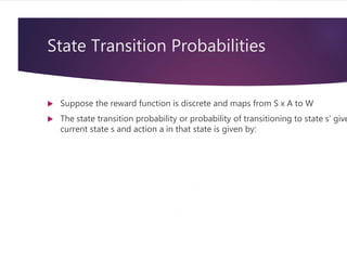
 State transition probabilities p(s’ | s, a). This is the probability distribution over the
state space given we take action a in state s
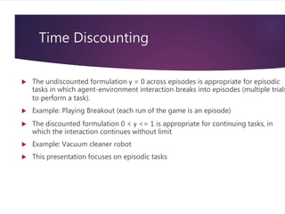
 Discount factor γ in [0, 1]
 Reward function R: S x A -> set of real numbers
 For simplicity, assume discrete rewards
 Finite MDP if both S and A are finite

19. Time Discounting
 The undiscounted formulation γ = 0 across episodes is appropriate for episodic
tasks in which agent-environment interaction breaks into episodes (multiple trials
to perform a task).
 Example: Playing Breakout (each run of the game is an episode)
 The discounted formulation 0 < γ <= 1 is appropriate for continuing tasks, in
which the interaction continues without limit
 Example: Vacuum cleaner robot
 This presentation focuses on episodic tasks

20. Agent-Environment Interaction (1)
 The agent and environment interact at each of a sequence of discrete time steps t
= {0, 1, 2, 3, …, T} where T can be infinite
 At each time step t, the agent receives some representation of the environment
state St in S and uses this to select an action At in the set A(St) of available actions
given that state
 One step later, the agent receives a numerical reward Rt+1 and finds itself in a new
state St+1

21. Agent-Environment Interaction (2)
 At each time step, the agent implements a stochastic policy or mapping from
states to probabilities of selecting each possible action
 The policy is denoted πt where πt(a | s) is the probability of taking action a when in
state s
 A policy is a stochastic rule by which the agent selects actions as a function of
states
 Reinforcement learning methods specify how the agent changes its policy using
its experience

22. Action Selection
 At time t, the agent tries to select an action to maximise the sum Gt of discounted
rewards received in the future

23. MDP Dynamics
 Given current state s and action a in that state, the probability of the next st
and the next reward r is given by:

24. State Transition Probabilities
 Suppose the reward function is discrete and maps from S x A to W
 The state transition probability or probability of transitioning to state s’ give
current state s and action a in that state is given by:

25. Expected Rewards
 The expected reward for a given state-action pair is given by:

26. State-Value Function (1)
 Value functions are defined with respect to particular policies because future
rewards depend on the agent’s actions
 Value functions give the expected return of a particular policy
 The value vπ(s) of a state s under a policy π is the expected return when starting in
state s and following the policy π from that state onwards

27. State-Value Function (2)
 The state-value function vπ(s) for the policy π is given below. Note that the value
of the terminal state (if any) is always zero.

28. Action-Value Function
 The value qπ(s, a) of taking action a in state s under a policy π is defined as the
expected return starting from s, taking the action a and thereafter following policy
π
 qπ is the action-value function for policy π

29. Bellman Equation (1)
 The equation expresses the relationship between the value of a state s and the
values of its successor states
 The value of the next state must equal the discounted value of the expected next
state, plus the reward expected along the way

30. Bellman Equation (2)
 The value of state s is the expected value of the sum of time-discounted rewards
(starting at current state) given current state s
 This is expected value of r plus the sum of time-discounted rewards (starting at
successor state) over all successor states s’ and all next rewards r and over all
possible actions a in current state s

31. Optimality
 A policy is defined to be better than or equal to another policy if its expected
return is greater than or equal to that of the other policy for all states
 There is always at least one optimal policy π* that is better than or equal to all
other policies
 All optimal policies share the same optimal state-value function v*, which gives
the maximum expected return for any state s over all possible policies
 All optimal policies share the same optimal action-value function q*, which gives
the maximum expected return for any state-action pair (s, a) over all possible
policies

32. Temporal-Difference
Learning
Chapter 6 – Reinforcement Learning: An Introduction
Playing Atari with Deep Reinforcement Learning
Asynchronous Methods for Deep Reinforcement Learning
David Silver’s Tutorial on Deep Reinforcement Learning

33. What is TD learning?
 Temporal-Difference learning = TD learning
 The prediction problem is that of estimating the value function for a policy π
 The control problem is the problem of finding an optimal policy π*
 Given some experience following a policy π, update estimate v of vπ for non-
terminal states occurring in that experience
 Given current step t, TD methods wait until the next time step to update V(St)
 Learn from partial returns

34. Value-based Reinforcement Learning
 We want to estimate the optimal value V*(s) or action-value function Q*(s, a) usin
a function approximator V(s; θ) or Q(s, a; θ) with parameters θ
 This function approximator can be any parametric supervised machine learning
model
 Recall that the optimal value is the maximum value achievable under any policy

35. Update Rule for TD(0)
 At time t + 1, TD methods immediately form a target Rt+1 + γ V(St+1) and make a
useful update with step size α using the observed reward Rt+1 and the estimate
V(St+1)
 The update is the step size times the difference between the target output and the
actual output

36. Update Rule Intuition
 The target output is a more accurate estimate of V(St) given the reward Rt+1 is
known
 The actual output is our current estimate of V(St)
 We simply take one step with our current value function estimate to get a more
accurate estimate of V(St) and then perform an update to move V(St) closer
towards the more accurate estimate (i.e. temporal difference)

37. Tabular TD(0) Algorithm

38. SARSA – On-policy TD Control
 SARSA = State-Action-Reward-State-Action
 Learn an action-value function instead of a state-value function
 qπ is the action-value function for policy π
 Q-values are the values qπ(s, a) for s in S, a in A
 SARSA experiences are used to update Q-values
 Use TD methods for the prediction problem

39. SARSA Update Rule
 We want to estimate qπ(s, a) for the current policy π, and for all states s and action
a
 The update rule is similar to that for TD(0) but we transition from state-action pair
to state-action pair, and learn the values of state-action pairs
 The update is performed after every transition from a non-terminal state St
 If St+1 is terminal, then Q(St+1, At+1) is zero
 The update rule uses (St, At, Rt+1, St+1, At+1)

40. SARSA Algorithm

41. Q-learning – Off-policy TD Control
 Similar to SARSA but off-policy updates
 The learned action-value function Q directly approximates the optimal action-
value function q* independent of the policy being followed
 In update rule, choose action a that maximises Q given St+1 and use the resulting
Q-value (i.e. estimated value given by optimal action-value function) plus the
observed reward as the target
 This method is off-policy because we do not have a fixed policy that maps from
states to actions. This is why At+1 is not used in the update rule

42. One-step Q-learning Algorithm

43. Epsilon-greedy Policy
 At each time step, the agent selects an action
 The agent follows the greedy strategy with probability 1 – epsilon
 The agent selects a random action with probability epsilon
 With Q-learning, the greedy strategy is the action a that maximises Q given St+1

44. Deep Q-Networks (DQN)
 Introduced deep reinforcement learning
 It is common to use a function approximator Q(s, a; θ) to approximate the action-
value function in Q-learning
 Deep Q-Networks is Q-learning with a deep neural network function approximator
called the Q-network
 Discrete and finite set of actions A
 Example: Breakout has 3 actions – move left, move right, no movement
 Uses epsilon-greedy policy to select actions

45. Q-Networks
 Core idea: We want the neural network to learn a non-linear hierarchy of features
or feature representation that gives accurate Q-value estimates
 The neural network has a separate output unit for each possible action, which
gives the Q-value estimate for that action given the input state
 The neural network is trained using mini-batch stochastic gradient updates and
experience replay

46. Experience Replay
 The state is a sequence of actions and observations st = x1, a1, x2, …, at-1, xt
 Store the agent’s experiences at each time step et = (st, at, rt, st+1) in a dataset D =
e1, ..., en pooled over many episodes into a replay memory
 In practice, only store the last N experience tuples in the replay memory and
sample uniformly from D when performing updates

47. State representation
 It is difficult to give the neural network a sequence of arbitrary length as input
 Use fixed length representation of sequence/history produced by a function ϕ(st)
 Example: The last 4 image frames in the sequence of Breakout gameplay

48. Q-Network Training
 Sample random mini-batch of experience tuples uniformly at random from D
 Similar to Q-learning update rule but:
 Use mini-batch stochastic gradient updates
 The gradient of the loss function for a given iteration with respect to the parameter θi is
the difference between the target value and the actual value is multiplied by the
gradient of the Q function approximator Q(s, a; θ) with respect to that specific
parameter
 Use the gradient of the loss function to update the Q function approximator

49. Loss Function Gradient Derivation

50. DQN Algorithm

51. Comments
 It was previously thought that the combination of simple online
reinforcement learning algorithms with deep neural networks was
fundamentally unstable
 The sequence of observed data (states) encountered by an online
reinforcement learning agent is non-stationary and online updates are
strongly correlated
 The technique of DQN is stable because it stores the agent’s data in
experience replay memory so that it can be randomly sampled from
different time-steps
 Aggregating over memory reduces non-stationarity and decorrelates
updates but limits methods to off-policy reinforcement learning algorithms
 Experience replay updates use more memory and computation per real
interaction than online updates, and require off-policy learning algorithms
that can update from data generated by an older policy

52. Policy Gradient Methods
Chapter 13 – Reinforcement Learning: An Introduction
Policy Gradient Lecture Slides from David Silver’s
Reinforcement Learning Course
David Silver’s Tutorial on Deep Reinforcement Learning

53. What are Policy Gradient Methods?
 Before: Learn the values of actions and then select actions based on their
estimated action-values. The policy was generated directly from the value
function
 We want to learn a parameterised policy that can select actions without
consulting a value function. The parameters of the policy are called policy
weights
 A value function may be used to learn the policy weights but this is not
required for action selection
 Policy gradient methods are methods for learning the policy weights using
the gradient of some performance measure with respect to the policy
weights

54. Policy-based Reinforcement Learning
 Search directly for the optimal policy π*
 Can use any parametric supervised machine learning model to learn policies π(a |s;
θ) where θ represents the learned parameters
 Recall that the optimal policy is the policy that achieves maximum future return

55. Notation
 Policy weight vector θ
 The policy is π(a | s, θ), which represents the probability that action a is taken in
state s with policy weight vector θ
 If using learned value functions, the value function’s weight vector is w
 Performance measure η(θ)
 Episodic case: η(θ) = vπ(s0)
 Performance is defined as the value of the start state under the parameterised
policy

56. Policy Approximation
 The policy can be parameterised in any way provided π(a | s, θ) is differentiable
with respect to its weights
 To ensure exploration, we generally require that the policy never becomes
deterministic and so π(a | s, θ) is in interval (0, 1)
 Assume discrete and finite set of actions
 Form parameterised numerical preferences h(s, a, θ) for each state-action pair
 Can use a deep neural network as the policy approximator
 Use softmax so that the most preferred actions in each state are given the highest
probability of being selected

57. Types of Policy Gradient Method
 Finite Difference Policy Gradient
 Monte Carlo Policy Gradient
 Actor-Critic Policy Gradient

58. Finite Difference Policy Gradient
 Compute the partial derivative of the performance measure η(θ) with respect
to θk using finite difference gradient approximation
 Compute performance measure η(θ)
 Perturb θ by small positive amount epsilon in the kth dimension and
compute performance measure η(θ + ukε) where uk is unit vector that is 1 in
kth component and 0 elsewhere
 The partial derivative is approximated by
( η(θ + ukε) - η(θ) ) / ε
 θk <- θk + α ( η(θ + ukε) - η(θ) ) / ε
 Perform gradient ascent using the partial derivative
 Simple, noisy and inefficient procedure that is sometimes effective

59. REINFORCE: Monte Carlo Policy Gradient
 We want a quantity that we can sample on each time step whose expectatio
equal to the gradient
 We can then perform stochastic gradient ascent with this quantity

60. REINFORCE Properties
 On-policy method
 Uses the complete return from time t, which includes all future rewards until the
end of the episode
 REINFORCE is thus a Monte Carlo algorithm and is only well-defined for the
episodic case with all updates made in retrospect after the episode is completed
 Note that the gradient of log x is the gradient of x divided by x by the chain rule

61. REINFORCE Algorithm

62. Actor-Critic Methods
 Methods that learn approximations to both policy and value functions are called
actor-critic methods
 Actor refers to the learned policy
 Critic refers to the learned value function, which is usually a state-value function
 The critic is bootstrapped – the state-values are updated using the estimated
state-values of subsequent states
 The number of steps in the actor-critic method controls the degree of
bootstrapping

63. One-step Actor-Critic Update Rules
 On-policy method
 The state-value function update rule is the TD(0) update rule
 The policy function update rule is shown below.
 For n-step Actor-Critic, simply replace Gt
(1) with Gt
(n)

64. One-step Actor-Critic Algorithm

65. Asynchronous
Reinforcement Learning
Asynchronous Methods for Deep Reinforcement
Learning

66. What is Asynchronous Reinforcement Learni
 Use asynchronous gradient descent to optimise controllers
 This is useful for deep reinforcement learning where the controllers are deep
neural networks, which take a long time to train
 Asynchronous gradient descent speeds up the learning process
 Can use one multi-core CPU to train deep neural networks asynchronously instead
of multiple GPUs

67. Parallelism (1)
 Asynchronously execute multiple agents in parallel on multiple instances of the
environment
 This parallelism decorrelates the agents’ data into a more stationary process since at
any given time-step, the agents will be experiencing a variety of different states
 This approach enables a larger spectrum of fundamental on-policy and off-policy
reinforcement learning algorithms to be applied robustly and effectively using deep
neural networks
 Use asynchronous actor-learners (i.e. agents). Think of each actor-learner as a thread
 Run everything on a single multi-core CPU to avoid communication costs of sending
gradients and parameters

68. Parallelism (2)
 Multiple actor-learners running in parallel are likely to be exploring different
parts of the environment
 We can explicitly use different exploration policies in each actor-learner to
maximise this diversity
 By running different exploration policies in different threads, the overall
changes made to the parameters by multiple actor-learners applying
updates in parallel are less likely to be correlated in time than a single agent
applying online updates

69. No Experience Replay
 No need for a replay memory. We instead rely on parallel actors employing
different exploration policies to perform the stabilising role undertaken by
experience replay in the DQN training algorithm
 Since we no longer rely on experience replay for stabilising learning, we are able
to use on-policy reinforcement learning methods to train neural networks in a
stable way

70. Asynchronous Algorithms
 Asynchronous one-step Q-learning
 Asynchronous one-step SARSA
 Asynchronous n-step Q-learning
 Asynchronous Advantage Actor-Critic (A3C)

71. Asynchronous one-step Q-learning
 Each thread interacts with its own copy of the environment and at each step,
computes the gradient of the Q-learning loss
 Use a globally shared and slowly changing target network with parameters
θ- when computing the Q-learning loss
 DQN uses a globally shared and slowly changing target network too – the
network is updated using a mini-batch of experience tuples drawn from
replay memory
 The gradients are accumulated over multiple time-steps before being
applied (similar to using mini-batches), which reduces chance of multiple
actor-learners overwriting each other’s updates

72. Exploration
 Giving each thread a different exploration policy helps improve robustness and
generally improves performance through better exploration
 Use epsilon-greedy exploration with epsilon periodically sampled from some
distribution by each thread

73. Asynchronous one-step Q-learning Algorithm

74. Asynchronous one-step SARSA
 This is the same algorithm as Asynchronous one-step Q-learning except the target
value used for Q(s, a) is different
 One-step SARSA uses r + γ Q(s’, a’; θ-) as the target value

75. n-step Q-learning
 So far we have been using one-step Q-learning
 One-step Q-learning updates the action value Q(s, a) towards r + γ maxa’ Q(s’, a’;
θ), which is the one-step return
 Obtaining a reward r only directly affects the value of the state-action pair (s, a)
that led to the reward
 The values of the other state-action pairs are affected only indirectly through the
updated value Q(s, a)
 This can make the learning process slow since many updates are required to
propagate a reward to the relevant preceding states and actions
 Use n-step returns to propagate the rewards faster

76. n-step Returns
 In n-step Q-learning, Q(s, a) is updated towards the n-step return:
 rt + γ rt+1 + … + γn-1 rt+n-1 + maxa γn Q(st+n, a)
 This results in a single reward directly affecting the values of n preceding state-
action pairs
 This makes the process of propagating rewards to relevant state-action pairs
potentially much more efficient
 One-step update for the last state, two-step update for the second last state, and
so on until n-step update for the nth last state
 Accumulated updates are applied in a single step

77. Asynchronous n-step Q-learning Algorithm

78. A3C
 Maintains a policy π(at| st; θ) and an estimate of the value function V(st; θv)
 n-step Actor-Critic method
 As with value-based methods, use parallel actor-learners and accumulate updates
to improve training stability
 In practice, the policy approximation and the value function share some
parameters
 Use a neural network that has one softmax output for the policy π(at| st; θ) and
one linear output for the value function V(st; θv) with all non-output parameters
shared

79. Advantage Definition
 For a one-step actor-critic method with a learned policy and a learned value
function, the advantage is defined as follows:
 A(at, st) = Q(at, st) – V(st)
 The quantity rt – V(st; θv) is an estimate of the advantage
 This estimate is used to scale the policy gradient in an actor-critic method
 The advantage estimate for a n-step actor-critic method is shown below:

80. A3C Algorithm

81. Summary
 Get faster training because of parallelism
 Can use on-policy reinforcement learning methods
 Diversity in exploration can lead to better performance than synchronous methods
 In practice, the on-policy A3C algorithm appears to be the best performing
asynchronous reinforcement learning method in terms of performance and
training speed