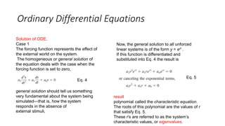
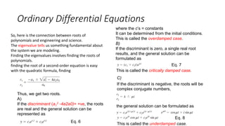
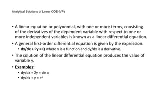
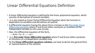
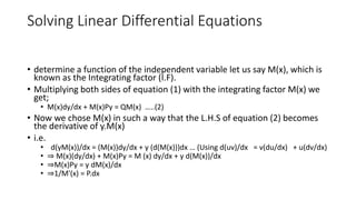
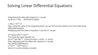
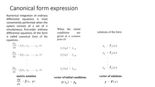
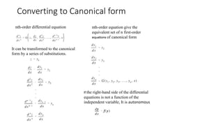
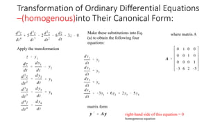
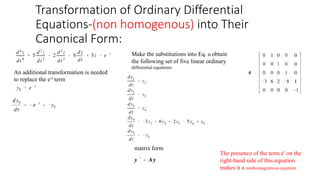
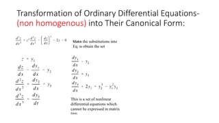
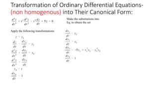
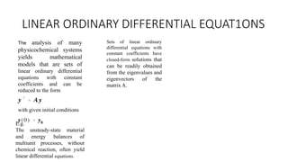
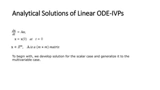
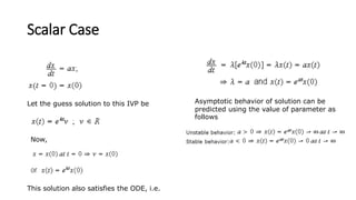
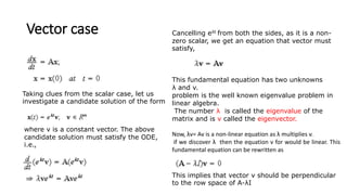
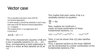
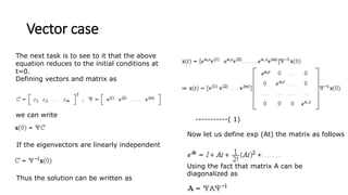
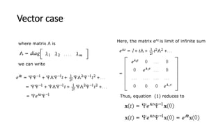
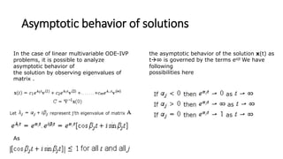
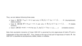
This document discusses analytical solutions of linear ordinary differential equation initial value problems (ODE-IVPs). It begins by introducing scalar and vector cases of linear ODE-IVPs. For the scalar case, it shows that the solution has the form of et. For the vector case, it shows that the solution has the form of eλtv, where λ are the eigenvalues of the coefficient matrix A and v are the corresponding eigenvectors. It then discusses how to determine the eigenvalues and eigenvectors by solving the characteristic equation of A. Finally, it expresses the general solution as a linear combination of the fundamental solutions eλtv, which must also satisfy the initial conditions.

1. MSME
MGN

2. Ordinary Differential Equations
• Part 1
• Initial Value Problems (ODE-IVPs) :
• Introduction
• Analytical Solutions of Linear ODE-IVPs
• Part 2
• basic concepts in Numerical solutions of ODE-IVP:
• step size and marching
• concept of implicit and explicit methods
• Taylor series based and Runge-Kutta methods
• Multi-step (predictor-corrector) approaches
• Stability of ODE-IVP solvers
• choice of step size and stability envelopes
• stiffness and variable step size implementation
• Introduction to solution methods for differential algebraic equations (DAEs),

3. Part 1
Introduction

4. Ordinary Differential Equations
• Ordinary differential equations are of
great significance in engineering
practice.
• This is because many physical laws are
understood in terms of the rate of
change of a quantity rather than the
magnitude of the quantity itself.
• Examples
• population-forecasting models (rate of
change of population)
• The acceleration of a falling body (rate of
change of velocity).
• Two types of problems are addressed:
initial-value and boundary-value
problems.

5. Ordinary Differential Equations
simple second-order system defined by the
following linear ordinary differential
equation
(or ODE)
where y and t are the dependent and
independent variables, respectively,
the a’s are constant coefficients, and F(t) is
the forcing function.
Eq 1 alternatively expressed as a pair
of first-order ODEs by defining a new variable z
Eq. 1
Equation 2 can be substituted along with its
derivative into Eq. 1 to remove the
second-derivative term.
This reduces the problem to solving
Eq. 2
Eq. 3
In a similar fashion, an nth-order linear ODE
can always be expressed as a system of n
first-order ODEs.

6. Ordinary Differential Equations
Solution of ODE.
Case 1
The forcing function represents the effect of
the external world on the system.
The homogeneous or general solution of
the equation deals with the case when the
forcing function is set to zero,
Eq. 4
general solution should tell us something
very fundamental about the system being
simulated—that is, how the system
responds in the absence of
external stimuli,
Now, the general solution to all unforced
linear systems is of the form y = ert .
If this function is differentiated and
substituted into Eq. 4 the result is
Eq. 5
result
polynomial called the characteristic equation.
The roots of this polynomial are the values of r
that satisfy Eq. 5.
These r’s are referred to as the system’s
characteristic values, or eigenvalues.

7. Ordinary Differential Equations
So, here is the connection between roots of
polynomials and engineering and science.
The eigenvalue tells us something fundamental about
the system we are modeling.
Finding the eigenvalues involves finding the roots of
polynomials.
finding the root of a second-order equation is easy
with the quadratic formula, finding
Thus, we get two roots.
A)
If the discriminant (a1
2 -4a2a0)= +ve, the roots
are real and the general solution can be
represented as
where the c’s = constants
It can be determined from the initial conditions.
This is called the overdamped case.
B)
If the discriminant is zero, a single real root
results, and the general solution can be
formulated as
This is called the critically damped case.
If the discriminant is negative, the roots will be
complex conjugate numbers,
C)
the general solution can be formulated as
This is called the underdamped case.
Eq. 6
Eq. 7
Eq. 8

8. Ordinary Differential Equations
• Equations 6,7 and 8 express the
possible ways that linear systems
respond dynamically.
• The exponential terms mean that the
solutions are capable of decaying
(negative real part) or growing
(positive real part) exponentially with
time (Fig. a).
• The sinusoidal terms (imaginary part)
mean that the solutions can oscillate
(Fig. b).
• If the eigenvalue has both real and
imaginary parts, the exponential and
sinusoidal shapes are combined (Fig.
c).

9. Ordinary Differential Equations
• Content available in
• Gupta, S. K.; Numerical Methods for Engineers. Wiley Eastern, New Delhi,
1995. (CH 5)
• Philips, G. M.,Taylor, P. J. ; Theory and Applications of Numerical Analysis (2nd
Ed.), Academic Press, 1996. (CH 13)
• Gilbert Strang, Linear Algebra and Its Applications (4th Ed.), Wellesley
Cambridge Press (2009). (CH 6 section 1)
• ref 1. Steven C. Chapra, Raymond P. Canale - Numerical Methods for
Engineers-McGraw-Hill Education (2014) ( part 7 )

10. Initial Value Problems (ODE-IVPs) :

11. Initial Value Problems (ODE-IVPs) :
• Introduction
• Newton’s second law to compute the velocity y of a falling parachutist as a function of time t by eq 1.
• --------- eq 1
• where g is the gravitational constant
• m is the mass
• c is a drag coefficient.
• Such equations, which are composed of an unknown function and its derivatives, are called differential
equations.
• Equation 1 is sometimes referred to as a rate equation because it expresses the rate of change of a variable as
a function of variables and parameters.
• Such equations play a fundamental role in engineering because many physical phenomena are best formulated
mathematically in terms of their rate of change.
• the quantity being differentiated, y, is called the dependent variable.
• The quantity with respect to which y is differentiated, t, is called the independent variable.
• When the function involves one independent variable, the equation is called an ordinary
differential equation (or ODE).
• This is in contrast to a partial differential equation (or PDE) that involves two or more independent
variables.

12. Initial Value Problems (ODE-IVPs) :
• Differential equations are also classified as to their order.
• For example, Eq 1 is called a first-order equation because the highest
derivative is a first derivative.
• A second-order equation would include a second derivative. For example, the
equation describing the position x of a mass-spring system with damping is
the second-order equation 2,
--------eq 2
• where c is a damping coefficient
• k is a spring constant.
• Similarly, an nth-order equation would include an nth derivative.

13. Initial Value Problems (ODE-IVPs) :
• Higher-order equations can be reduced to a system of first-order equations.
• For Eq. 2, this is done by defining a new variable y, where
• which itself can be differentiated to yield
• Hence equation reduces to -----eq 3
• These are a pair of first-order equations that are equivalent to the original
second-order equation.
• Because other nth-order differential equations can be similarly reduced.

14. Solution of the ODE
• Non-computer Methods for Solving ODEs

15. Non-computer Methods for Solving ODEs
• Without computers, ODEs are usually solved with analytical integration
techniques. For example, Eq. 1 could be multiplied by dt and integrated to
yield
eq 4
• The right-hand side of this equation is called an indefinite integral because
the limits of integration are unspecified.
• An analytical solution for Eq. 4 is obtained if the indefinite integral can be
evaluated exactly in equation form.
• For example, recall that for the falling parachutist problem, Eq. 4 was
solved analytically by assuming y = 0 at t = 0):

16. Non-computer Methods for Solving ODEs
For
the time being, the important fact is that exact solutions for many ODEs of practical
importance are not available. As is true for most situations discussed in other parts of
this book, numerical methods offer the only viable alternative for these cases.

17. Analytical Solutions of Linear ODE-IVPs

18. Analytical Solutions of Linear ODE-IVPs
• A linear equation or polynomial, with one or more terms, consisting
of the derivatives of the dependent variable with respect to one or
more independent variables is known as a linear differential equation.
• A general first-order differential equation is given by the expression:
• dy/dx + Py = Q where y is a function and dy/dx is a derivative.
• The solution of the linear differential equation produces the value of
variable y.
• Examples:
• dy/dx + 2y = sin x
• dy/dx + y = ex

19. Linear Differential Equations Definition
• A linear differential equation is defined by the linear polynomial equation, which
consists of derivatives of several variables.
• It is also stated as Linear Partial Differential Equation when the function is
dependent on variables and derivatives are partial.
• A differential equation having the above form is known as the first-order linear
differential equation where P and Q are either constants or functions of the
independent variable (in this case x) only.
• Also, the differential equation of the form,
• dy/dx + Py = Q ------ eq 1
• is a first-order linear differential equation where P and Q are either constants
or functions of y (independent variable) only.
• To find linear differential equations solution, we have to derive the general form
or representation of the solution.

20. Solving Linear Differential Equations
• determine a function of the independent variable let us say M(x), which is
known as the Integrating factor (I.F).
• Multiplying both sides of equation (1) with the integrating factor M(x) we
get;
• M(x)dy/dx + M(x)Py = QM(x) …..(2)
• Now we chose M(x) in such a way that the L.H.S of equation (2) becomes
the derivative of y.M(x)
• i.e.
• d(yM(x))/dx = (M(x))dy/dx + y (d(M(x)))dx … (Using d(uv)/dx = v(du/dx) + u(dv/dx)
• ⇒ M(x)(dy/dx) + M(x)Py = M (x) dy/dx + y d(M(x))/dx
• ⇒M(x)Py = y dM(x)/dx
• ⇒1/M'(x) = P.dx

21. Solving Linear Differential Equations
Integrating both sides with respect to x, we get;
log M (x) = ∫Pdx (As∫f′(x)f(x))=logf(x)
⇒ M(x) = e∫Pdx I.F
Now, using this value of the integrating factor, we can find out the solution of our first order linear
differential equation.
Multiplying both the sides of equation (1) by the I.F. we get
e∫Pdxdy/dx+yPe∫Pdx=Qe∫Pdx
This could be easily rewritten as:
d(y.e∫Pdx)dx=Qe∫Pdx (Using d(uv)dx=v. du/dx + u. dv/dx)
Now integrating both the sides with respect to x, we get:
∫d(y.e∫Pdx)=∫Qe∫Pdxdx+c
y=1/e∫Pdx * (∫Qe∫Pdxdx+c)
where C is some arbitrary constant.

22. How to Solve First Order Linear Differential
Equation

23. How to Solve First Order Linear Differential
Equation

26. Canonical form expression
Numerical integration of ordinary
differential equations is most
conveniently performed when the
system consists of a set of n
simultaneous first-order ordinary
differential equations of the form
is called canonical form of the
equations.
When the initial
conditions are
given at a common
point x0
solutions of the form
matrix notation vector of initial conditions vector of solutions

27. Converting to Canonical form
nth-order differential equation
It can be transformed to the canonical
form by a series of substitutions.
nth-order equation give the
equivalent set of n first-order
equations of canonical form
If the right-hand side of the differential
equations is not a function of the
independent variable, It is autonomous

28. Transformation of Ordinary Differential Equations
–(homogenous)into Their Canonical Form:
Apply the transformation
Make these substitutions into Eq.
(a) to obtain the following four
equations:
matrix form
where matrix A
right-hand side of this equation = 0
homogeneous equation

30. Transformation of Ordinary Differential
Equations-(non homogenous) into Their
Canonical Form:
An additional transformation is needed
to replace the e-t term
Make the substitutions into Eq. to obtain
the following set of five linear ordinary
differential equations:
matrix form
The presence of the term e' on the
right-hand side of this equation
makes it a nonhomogeneous equation

31. Transformation of Ordinary Differential Equations-
(non homogenous) into Their Canonical Form:
Make the substitutions into
Eq. to obtain the set
This is a set of nonlinear
differential equations which
cannot be expressed in matrix
form.

32. Transformation of Ordinary Differential Equations-
(non homogenous) into Their Canonical Form:
Apply the following transformations
Make the substitutions into
Eq. to obtain the set

33. LINEAR ORDINARY DIFFERENTIAL EQUAT1ONS
The analysis of many
physicochemical systems
yields mathematical
models that are sets of
linear ordinary differential
equations with constant
coefficients and can be
reduced to the form
with given initial conditions
E.g.
The unsteady-state material
and energy balances of
multiunit processes, without
chemical reaction, often yield
linear differential equations.
Sets of linear ordinary
differential equations with
constant coefficients have
closed-form solutions that
can be readily obtained
from the eigenvalues and
eigenvectors of the
matrix A.

34. Analytical Solutions of Linear ODE-IVPs
• Before developing numerical schemes for solving ODE IVPs, we
consider a special sub-class of ODE -IVPs, i.e. linear multi-variable
ODE-IVPs, which can be solved analytically.
• The reason for considering this sub-class is two fold:
• A set of nonlinear ODE-IVPs can often be approximated locally as a set of
linear ODE-IVPs using Taylor series approximation. Thus, it provides insights
into how solutions of a nonlinear ODE-IVP evolve for small perturbations.
• Since the solution of a linear ODE-IVP can be constructed analytically, it
proves to be quite useful while understanding stability behavior of numerical
schemes for solving ODE-IVPs.
• Consider the problem of solving simultaneous linear ODE-IVP

35. Analytical Solutions of Linear ODE-IVPs
To begin with, we develop solution for the scalar case and generalize it to the
multivariable case.

36. Scalar Case
Let the guess solution to this IVP be
Now,
This solution also satisfies the ODE, i.e.
Asymptotic behavior of solution can be
predicted using the value of parameter as
follows

37. Vector case
where v is a constant vector. The above
candidate solution must satisfy the ODE,
i.e.,
Taking clues from the scalar case, let us
investigate a candidate solution of the form
Cancelling eλt from both the sides, as it is a non-
zero scalar, we get an equation that vector must
satisfy,
This fundamental equation has two unknowns
λ and v.
problem is the well known eigenvalue problem in
linear algebra.
The number λ is called the eigenvalue of the
matrix and is v called the eigenvector.
Now, λv= Av is a non-linear equation as λ multiplies v.
if we discover λ then the equation v for would be linear. This
fundamental equation can be rewritten as
This implies that vector v should be perpendicular
to the row space of A-λI

38. Vector case
This is possible only when rows of A-λI
are linearly dependent.
In other words, λ should be selected in such a way
that rows of A-λI become linearly dependent,
i.e., is singular.
This implies that λ is an eigenvalue of A
if and only if
This is the characteristic equation of A and
it has m possible solutions λ1, λ2,…. λm.
Thus, corresponding to each eigenvalue λi,
there is a vector vi that satisfies (A-λI) vi
=0
This implies that each vector eλitvi is a
candidate solution to equation
Now, suppose we construct a
vector as lineal combination of these
fundamental solutions, i.e.
Then, it can be shown that x(t) also satisfies
equation.
Thus, a general solution to the linear ODEIVP
can be constructed as a linear combination of the
fundamental solutions eλitvi .

39. Vector case
The next task is to see to it that the above
equation reduces to the initial conditions at
t=0.
Defining vectors and matrix as
we can write
If the eigenvectors are linearly independent
Thus the solution can be written as
Now let us define exp (At) the matrix as follows
Using the fact that matrix A can be
diagonalized as
-----------( 1)

40. Vector case
where matrix Λ is
we can write
Here, the matrix eΛt is limit of infinite sum
Thus, equation (1) reduces to

41. Asymptotic behavior of solutions
In the case of linear multivariable ODE-IVP
problems, it is possible to analyze
asymptotic behavior of
the solution by observing eigenvalues of
matrix .
As
the asymptotic behavior of the solution x(t) as
t∞ is governed by the terms eαjt We have
following
possibilities here

43. • Part 2
• basic concepts in Numerical solutions of ODE-IVP:
• step size and marching
• concept of implicit and explicit methods
• Taylor series based and Runge-Kutta methods
• Multi-step (predictor-corrector) approaches
• Stability of ODE-IVP solvers
• choice of step size and stability envelopes
• stiffness and variable step size implementation
• Introduction to solution methods for differential algebraic equations (DAEs),

44. Numerical Solution Schemes: Basic Concepts
Marching in Time
denote the true / actual solution of the above ODE-IVP.
In general, for a nonlinear ODE, it is seldom possible to obtain the true solution analytically.
The aim of numerical methods is to find an approximate solution numerically.
Let
Let
be a sequence of numbers such that
, we attempt to approximate the sequence of vectors
Thus, in order to integrate over a large interval we solve a sequence of ODE-IVPs
Sub problems

45. Marching in Time
Instead of attempting to approximate the function
which is defined for all values of such that
we attempt to approximate the sequence of vectors
we solve a sequence of ODE-IVPs subproblems

46. Marching in Time
each defined over a smaller interval
This generates a sequence of approximate solution vectors
The difference
is referred to as the integration step size or the integration interval.
Two possibilities can be considered regarding the choice of the sequence
1. Fixed integration interval: The numbers tn are equispaced, i.e., tn = nh for some h>0
2. Variable size integration intervals

47. Two Solution Approaches : Implicit and Explicit
There are two basic approaches to numerical integrations. To understand these approaches,
consider the integration of the equation (ODEs) over the interval
using Euler's method.
Let us also assume that the numbers tn are equi-spaced and h is the integration stepsize.
Explicit Euler method:If the integration interval is small,
The new value x(n+1) is a function of x only the past value of i.e., x(n) .
This type of numerical scheme is called explicit as it does not involve iterative calculations
while moving forward in time.

48. Implicit Euler method:
Each of the above equation has to be solved by iterative method.
For example if we use successive substitution method for solving the resulting nonlinear equation(s), the
algorithm is summarized as
This type of numerical scheme is called implicit
as it involves iterative calculations while moving forward in
time.

49. Taylor series based and Runge-Kutta methods
Consider a simple scalar case
Suppose we know the exact solution
and the integration step h size is selected sufficiently small,
then we can compute
using Taylor series expansion with respect to
independent variable as
The various derivatives in the above series can be
calculated using the differential equation, as
Now, the exact differential of f(x,t)
we can write

50. Taylor series based and Runge-Kutta methods
Let us now suppose that, instead of actual solution
x*(n) , we have available an approximation to x*(n) ,
denoted as x (n) . With this information, we can
construct
Further approximation by truncating the infinite series.
If the Taylor series is
truncated after hk the term involving , then the Taylor's series
method is said to be of order k .
Order 1(Euler explicit formula)
Order 2
Taylor's series methods are useful starting points for understanding more sophisticated methods,
but are not of much computational use. First order method is too inaccurate and the higher order
methods require calculation of a lot of partial derivatives.

51. Univariate Runge-Kutta (R-K) Methods
Runge-Kutta methods duplicate the accuracy of the
Taylor series methods, but do not require the
calculation of higher partial derivatives.
For example, consider the second order method that
uses the formula
The real numbers α, β, a, and b are chosen such that the RHS of
(RK method) approximates the RHS of
Taylor series method of order 2. To see how this is achieved, let
k2 be represented as where
and
consider the Taylor series expansion of the function k2
about

52. Univariate Runge-Kutta (R-K) Methods
where subscript denotes that the corresponding derivatives have been computed at
Substituting the Taylor series expansion in equation
Order 2
Comparing eqn1 and eqn3, we arrive at the following set of constraints on the parameters
-----eqn3
-----eqn1
Thus, there are 4 unknowns and 3 equations and we can choose one variable arbitrarily. Let us
select variable as the one that can be set arbitrarily. With this choice, we have

53. Univariate Runge-Kutta (R-K) Methods
together with the condition
Thus, the general 2nd order algorithm can be stated as
Heun's modified algorithm: Set b = 1/2.
Modified Euler-Cauchy Method: Set b = 1.
It must be emphasized that eqn4. and eqn1 do not give identical results. However, if we start from
the same x(n), then x(n+1) given by eqn1 and eqn4 would differ only by

54. Univariate Runge-Kutta (R-K) Methods
The third and higher order methods can be derived in an analogous manner. The general
computational form of the third order method can be expressed as follows
The parameters are chosen such that the RHS of (eqn5) approximates the RHS
of Taylor series method of order 3.

55. Multivariate R-K Methods
The most commonly used fourth order R-K method for one variable can be stated as
Now, suppose we want to use this method for solving simultaneous ODE-IVPs

56. Multivariate R-K Methods
Then, the above algorithm can be modified as follows

57. numerical method
According to this equation, the slope estimate of Φ is
used to extrapolate from an old value yi to a new value
yi+1 over a distance h.
This formula can be applied step by step to compute out
into the future and, hence, trace out the trajectory of the
solution.
Graphical depiction of a onestep method.