Full Download : https://goo.gl/ixWZLs Fox And Mcdonald's Introduction To Fluid Mechanics 8th Edition Pritchard Solutions Manual

1. Problem 1.15 [Difficulty: 5]
Given: Data on sky diver: M 70 kg⋅= kvert 0.25
N s
2
⋅
m
2
⋅= khoriz 0.05
N s
2
⋅
m
2
⋅= U0 70
m
s
⋅=
Find: Plot of trajectory.
Solution: Use given data; integrate equation of motion by separating variables.
Treat the sky diver as a system; apply Newton's 2nd law in horizontal and vertical directions:
Vertical: Newton's 2nd law for the sky diver (mass M) is (ignoring buoyancy effects): M
dV
dt
⋅ M g⋅ kvert V
2
⋅−= (1)
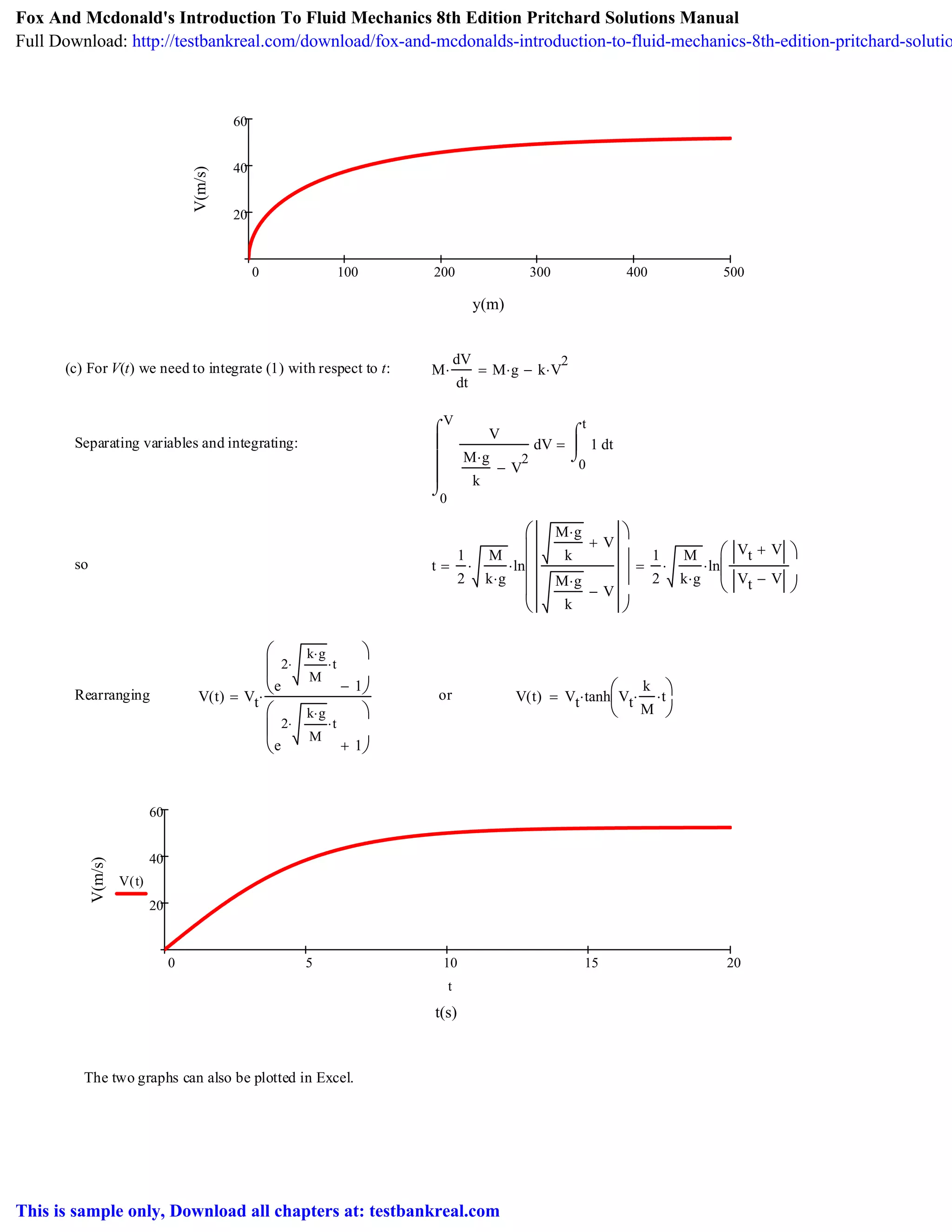
For V(t) we need to integrate (1) with respect to t:
Separating variables and integrating:
0
V
V
V
M g⋅
kvert
V
2
−
⌠
⎮
⎮
⎮
⎮
⌡
d
0
t
t1
⌠
⎮
⌡
d=
so t
1
2
M
kvert g⋅
⋅ ln
M g⋅
kvert
V+
M g⋅
kvert
V−
⎛
⎜
⎜
⎜
⎜
⎝
⎞
⎟
⎟
⎠
⋅=
Rearranging o
r
V t( )
M g⋅
kvert
e
2
kvert g⋅
M
⋅ t⋅
1−
⎛
⎜
⎜
⎝
⎞
⎠
e
2
kvert g⋅
M
⋅ t⋅
1+
⎛
⎜
⎜
⎝
⎞
⎠
⋅= so V t( )
M g⋅
kvert
tanh
kvert g⋅
M
t⋅
⎛
⎜
⎝
⎞
⎠
⋅=
For y(t) we need to integrate again:
dy
dt
V= or y tV
⌠
⎮
⌡
d=
y t( )
0
t
tV t( )
⌠
⎮
⌡
d=
0
t
t
M g⋅
kvert
tanh
kvert g⋅
M
t⋅
⎛
⎜
⎝
⎞
⎠
⋅
⌠
⎮
⎮
⎮
⌡
d=
M g⋅
kvert
ln cosh
kvert g⋅
M
t⋅
⎛
⎜
⎝
⎞
⎠
⎛
⎜
⎝
⎞
⎠
⋅=
y t( )
M g⋅
kvert
ln cosh
kvert g⋅
M
t⋅
⎛
⎜
⎝
⎞
⎠
⎛
⎜
⎝
⎞
⎠
⋅=
Fox And Mcdonald's Introduction To Fluid Mechanics 8th Edition Pritchard Solutions Manual
Full Download: http://testbankreal.com/download/fox-and-mcdonalds-introduction-to-fluid-mechanics-8th-edition-pritchard-solutio
This is sample only, Download all chapters at: testbankreal.com

2. After the first few seconds we reach steady state:
0 1 2 3 4 5
10
20
30
t(s)
y(m)
y t( )
t
0 20 40 60
200
400
600
t(s)
y(m)
y t( )
t
Horizontal: Newton's 2nd law for the sky diver (mass M) is: M
dU
dt
⋅ khoriz− U
2
⋅= (2)
For U(t) we need to integrate (2) with respect to t:
Separating variables and integrating:
U0
U
U
1
U
2
⌠
⎮
⎮
⎮
⌡
d
0
t
t
khoriz
M
−
⌠
⎮
⎮
⌡
d= so
khoriz
M
− t⋅
1
U
−
1
U0
+=
Rearranging U t( )
U0
1
khoriz U0⋅
M
t⋅+
=
For x(t) we need to integrate again:
dx
dt
U= or x tU
⌠
⎮
⌡
d=
x t( )
0
t
tU t( )
⌠
⎮
⌡
d=
0
t
t
U0
1
khoriz U0⋅
M
t⋅+
⌠
⎮
⎮
⎮
⎮
⌡
d=
M
khoriz
ln
khoriz U0⋅
M
t⋅ 1+
⎛
⎜
⎝
⎞
⎠
⋅=
x t( )
M
khoriz
ln
khoriz U0⋅
M
t⋅ 1+
⎛
⎜
⎝
⎞
⎠
⋅=

3. 0 20 40 60
0.5
1
1.5
2
t(s)
x(km)
Plotting the trajectory:
0 1 2 3
3−
2−
1−
x(km)
y(km)
These plots can also be done in Excel.

4. Problem 1.16 [Difficulty: 3]
Given: Long bow at range, R = 100 m. Maximum height of arrow is h = 10 m. Neglect air resistance.
Find: Estimate of (a) speed, and (b) angle, of arrow leaving the bow.
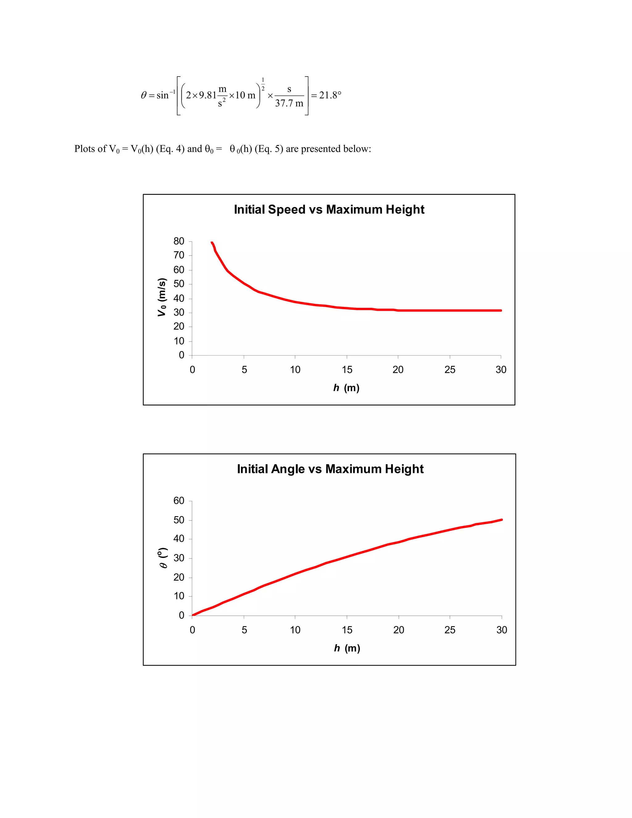
Plot: (a) release speed, and (b) angle, as a function of h
Solution: Let V u i v j V i j)0 0 0= + = +0 0 0(cos sinθ θ
ΣF m mgy
dv
dt
= = − , so v = v0 – gt, and tf = 2tv=0 = 2v0/g
Also, mv
dv
dy
mg, v dv g dy, 0
v
2
gh0
2
= − = − − = −
Thus h v 2g0
2
= (1)
ΣF m
du
dt
0, so u u const, and R u t
2u v
g
0 0 f
0 0
x = = = = = = (2)
From Eq. 1: v 2gh0
2
= (3)
From Eq. 2: u
gR
2v
gR
2 2gh
u
gR
8h
0
0
0
2
2
= = ∴ =
Then
2
1
2
0
2
2
0
2
0
2
0
8
2and2
8 ⎟⎟
⎠
⎞
⎜⎜
⎝
⎛
+=+=+=
h
gR
ghVgh
h
gR
vuV (4)
s
m
7.37
m10
1
m100
s
m
8
81.9
m10
s
m
81.92
2
1
22
220 =⎟⎟
⎠
⎞
⎜⎜
⎝
⎛
××+××=V
From Eq. 3: v 2gh V sin sin
2gh
V
0 0
1
0
= = = −
θ θ, (5)
R
V0
θ0
y
x
h

5. °=
⎥
⎥
⎦
⎤
⎢
⎢
⎣
⎡
×⎟
⎠
⎞
⎜
⎝
⎛
××= −
8.21
m37.7
s
m10
s
m
81.92sin
2
1
2
1
θ
Plots of V0 = V0(h) (Eq. 4) and θ0 = θ 0(h) (Eq. 5) are presented below:
Initial Speed vs Maximum Height
0
10
20
30
40
50
60
70
80
0 5 10 15 20 25 30
h (m)
V0(m/s)
Initial Angle vs Maximum Height
0
10
20
30
40
50
60
0 5 10 15 20 25 30
h (m)
θ(o
)

6. Problem 1.17 [Difficulty: 2]
Given: Basic dimensions M, L, t and T.
Find: Dimensional representation of quantities below, and typical units in SI and English systems.
Solution:
(a) Power Power
Energy
Time
Force Distance×
Time
==
F L⋅
t
=
From Newton's 2nd law Force Mass Acceleration×= so F
M L⋅
t
2
=
Hence Power
F L⋅
t
=
M L⋅ L⋅
t
2
t⋅
=
M L
2
⋅
t
3
=
kg m
2
⋅
s
3
slug ft
2
⋅
s
3
(b) Pressure Pressure
Force
Area
=
F
L
2
=
M L⋅
t
2
L
2
⋅
=
M
L t
2
⋅
=
kg
m s
2
⋅
slug
ft s
2
⋅
(c) Modulus of elasticity Pressure
Force
Area
=
F
L
2
=
M L⋅
t
2
L
2
⋅
=
M
L t
2
⋅
=
kg
m s
2
⋅
slug
ft s
2
⋅
(d) Angular velocity AngularVelocity
Radians
Time
=
1
t
=
1
s
1
s
(e) Energy Energy Force Distance×= F L⋅=
M L⋅ L⋅
t
2
=
M L
2
⋅
t
2
=
kg m
2
⋅
s
2
slug ft
2
⋅
s
2
(f) Moment of a force MomentOfForce Force Length×= F L⋅=
M L⋅ L⋅
t
2
=
M L
2
⋅
t
2
=
kg m
2
⋅
s
2
slug ft
2
⋅
s
2
(g) Momentum Momentum Mass Velocity×= M
L
t
⋅=
M L⋅
t
=
kg m⋅
s
slug ft⋅
s
(h) Shear stress ShearStress
Force
Area
=
F
L
2
=
M L⋅
t
2
L
2
⋅
=
M
L t
2
⋅
=
kg
m s
2
⋅
slug
ft s
2
⋅
(i) Strain Strain
LengthChange
Length
=
L
L
= Dimensionless
(j) Angular momentum AngularMomentum Momentum Distance×=
M L⋅
t
L⋅=
M L
2
⋅
t
=
kg m
2
⋅
s
slugs ft
2
⋅
s

7. Problem 1.18 [Difficulty: 2]
Given: Basic dimensions F, L, t and T.
Find: Dimensional representation of quantities below, and typical units in SI and English systems.
Solution:
(a) Power Power
Energy
Time
Force Distance×
Time
==
F L⋅
t
=
N m⋅
s
lbf ft⋅
s
(b) Pressure Pressure
Force
Area
=
F
L
2
=
N
m
2
lbf
ft
2
(c) Modulus of elasticity Pressure
Force
Area
=
F
L
2
=
N
m
2
lbf
ft
2
(d) Angular velocity AngularVelocity
Radians
Time
=
1
t
=
1
s
1
s
(e) Energy Energy Force Distance×= F L⋅= N m⋅ lbf ft⋅
(f) Momentum Momentum Mass Velocity×= M
L
t
⋅=
From Newton's 2nd law Force Mass Acceleration×= so F M
L
t
2
⋅= or M
F t
2
⋅
L
=
Hence Momentum M
L
t
⋅=
F t
2
⋅ L⋅
L t⋅
= F t⋅= N s⋅ lbf s⋅
(g) Shear stress ShearStress
Force
Area
=
F
L
2
=
N
m
2
lbf
ft
2
(h) Specific heat SpecificHeat
Energy
Mass Temperature×
=
F L⋅
M T⋅
=
F L⋅
F t
2
⋅
L
⎛
⎜
⎝
⎞
⎠
T⋅
=
L
2
t
2
T⋅
=
m
2
s
2
K⋅
ft
2
s
2
R⋅
(i) Thermal expansion coefficient ThermalExpansionCoefficient
LengthChange
Length
Temperature
=
1
T
=
1
K
1
R
(j) Angular momentum AngularMomentum Momentum Distance×= F t⋅ L⋅= N m⋅ s⋅ lbf ft⋅ s⋅

8. Problem 1.19 [Difficulty: 1]
Given: Viscosity, power, and specific energy data in certain units
Find: Convert to different units
Solution:
Using data from tables (e.g. Table G.2)
(a) 1
m
2
s
⋅ 1
m
2
s
⋅
1
12
ft⋅
0.0254 m⋅
⎛
⎜
⎜
⎝
⎞
⎠
2
×= 10.76
ft
2
s
⋅=
(b) 100 W⋅ 100 W⋅
1 hp⋅
746 W⋅
×= 0.134 hp⋅=
(c) 1
kJ
kg
⋅ 1
kJ
kg
⋅
1000 J⋅
1 kJ⋅
×
1 Btu⋅
1055 J⋅
×
0.454 kg⋅
1 lbm⋅
×= 0.43
Btu
lbm
⋅=

9. Problem 1.10 [Difficulty: 4]
NOTE: Drag formula is in error: It should be:
FD 3 π⋅ V⋅ d⋅=
Mg
FD = 3πVd
a = dV/dt
Given: Data on sphere and formula for drag.
Find: Diameter of gasoline droplets that take 1 second to fall 10 in.
Solution: Use given data and data in Appendices; integrate equation of
motion by separating variables.
The data provided, or available in the Appendices, are:
μ 4.48 10
7−
×
lbf s⋅
ft
2
⋅= ρw 1.94
slug
ft
3
⋅= SGgas 0.72= ρgas SGgas ρw⋅= ρgas 1.40
slug
ft
3
⋅=
Newton's 2nd law for the sphere (mass M) is (ignoring buoyancy effects) M
dV
dt
⋅ M g⋅ 3 π⋅ μ⋅ V⋅ d⋅−=
dV
g
3 π⋅ μ⋅ d⋅
M
V⋅−
dt=
so
Integrating twice and using limits V t( )
M g⋅
3 π⋅ μ⋅ d⋅
1 e
3− π⋅ μ⋅ d⋅
M
t⋅
−
⎛
⎜
⎝
⎞
⎠⋅= x t( )
M g⋅
3 π⋅ μ⋅ d⋅
t
M
3 π⋅ μ⋅ d⋅
e
3− π⋅ μ⋅ d⋅
M
t⋅
1−
⎛
⎜
⎝
⎞
⎠⋅+
⎡
⎢
⎢
⎣
⎤
⎥
⎥
⎦
⋅=
Replacing M with an expression involving diameter d M ρgas
π d
3
⋅
6
⋅= x t( )
ρgas d
2
⋅ g⋅
18 μ⋅
t
ρgas d
2
⋅
18 μ⋅
e
18− μ⋅
ρgas d
2
⋅
t⋅
1−
⎛
⎜
⎜
⎝
⎞
⎠⋅+
⎡⎢
⎢
⎢
⎣
⎤⎥
⎥
⎥
⎦
⋅=
This equation must be solved for d so that x 1 s⋅( ) 10 in⋅= . The answer can be obtained from manual iteration, or by using
Excel's Goal Seek.
d 4.30 10
3−
× in⋅=
0 0.025 0.05 0.075 0.1
0.25
0.5
0.75
1
t (s)
x(in)
0 0.25 0.5 0.75 1
2.5
5
7.5
10
t (s)
x(in)
Note That the particle quickly reaches terminal speed, so that a simpler approximate solution would be to solve Mg = 3πµVd for d,
with V = 0.25 m/s (allowing for the fact that M is a function of d)!

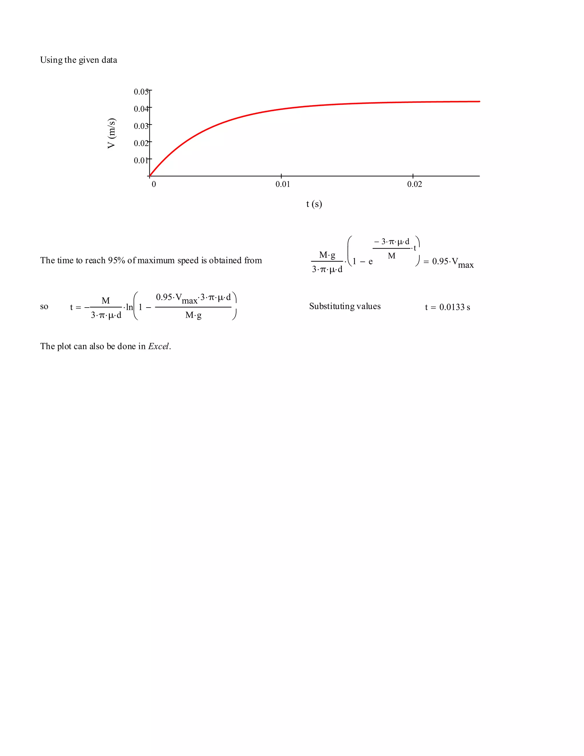
10. Problem 1.11 [Difficulty: 3]
Given: Data on sphere and formula for drag.
Find: Maximum speed, time to reach 95% of this speed, and plot speed as a function of time.
Solution: Use given data and data in Appendices, and integrate equation of motion by separating variables.
The data provided, or available in the Appendices, are:
ρair 1.17
kg
m
3
⋅= μ 1.8 10
5−
×
N s⋅
m
2
⋅= ρw 999
kg
m
3
⋅= SGSty 0.016= d 0.3 mm⋅=
Then the density of the sphere is ρSty SGSty ρw⋅= ρSty 16
kg
m
3
=
The sphere mass is M ρSty
π d
3
⋅
6
⋅= 16
kg
m
3
⋅ π×
0.0003 m⋅( )
3
6
×= M 2.26 10
10−
× kg=
Newton's 2nd law for the steady state motion becomes (ignoring buoyancy effects) M g⋅ 3 π⋅ V⋅ d⋅=
so
Vmax
M g⋅
3 π⋅ μ⋅ d⋅
=
1
3 π⋅
2.26 10
10−
×× kg⋅ 9.81×
m
s
2
⋅
m
2
1.8 10
5−
× N⋅ s⋅
×
1
0.0003 m⋅
×= Vmax 0.0435
m
s
=
Newton's 2nd law for the general motion is (ignoring buoyancy effects) M
dV
dt
⋅ M g⋅ 3 π⋅ μ⋅ V⋅ d⋅−=
Mg
FD = 3πVd
a = dV/dt
so
dV
g
3 π⋅ μ⋅ d⋅
M
V⋅−
dt=
Integrating and using limits V t( )
M g⋅
3 π⋅ μ⋅ d⋅
1 e
3− π⋅ μ⋅ d⋅
M
t⋅
−
⎛
⎜
⎝
⎞
⎠⋅=

11. Using the given data
0 0.01 0.02
0.01
0.02
0.03
0.04
0.05
t (s)
V(m/s)
The time to reach 95% of maximum speed is obtained from
M g⋅
3 π⋅ μ⋅ d⋅
1 e
3− π⋅ μ⋅ d⋅
M
t⋅
−
⎛
⎜
⎝
⎞
⎠⋅ 0.95 Vmax⋅=
so t
M
3 π⋅ μ⋅ d⋅
− ln 1
0.95 Vmax⋅ 3⋅ π⋅ μ⋅ d⋅
M g⋅
−
⎛
⎜
⎝
⎞
⎠
⋅= Substituting values t 0.0133 s=
The plot can also be done in Excel.

12. Problem 1.12 [Difficulty: 3]
mg
kVt
Given: Data on sphere and terminal speed.
Find: Drag constant k, and time to reach 99% of terminal speed.
Solution: Use given data; integrate equation of motion by separating variables.
The data provided are: M 1 10
13−
× slug⋅= Vt 0.2
ft
s
⋅=
Newton's 2nd law for the general motion is (ignoring buoyancy effects) M
dV
dt
⋅ M g⋅ k V⋅−= (1)
Newton's 2nd law for the steady state motion becomes (ignoring buoyancy effects) M g⋅ k Vt⋅= so k
M g⋅
Vt
=
k 1 10
13−
× slug⋅ 32.2×
ft
s
2
⋅
s
0.2 ft⋅
×
lbf s
2
⋅
slug ft⋅
×= k 1.61 10
11−
×
lbf s⋅
ft
⋅=
dV
g
k
M
V⋅−
dt=
To find the time to reach 99% of Vt, we need V(t). From 1, separating variables
Integrating and using limits t
M
k
− ln 1
k
M g⋅
V⋅−⎛
⎜
⎝
⎞
⎠
⋅=
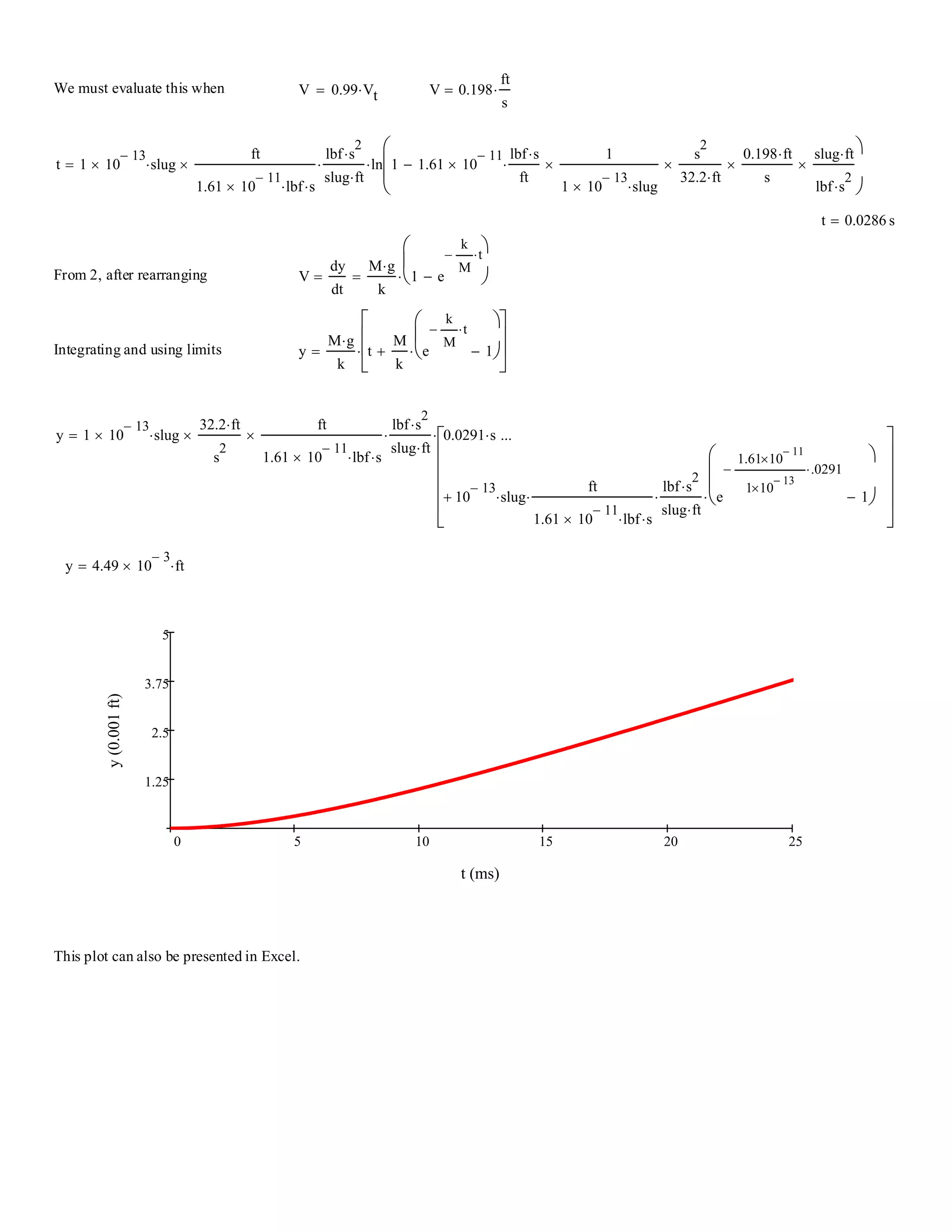
We must evaluate this when V 0.99 Vt⋅= V 0.198
ft
s
⋅=
t 1− 10
13−
× slug⋅
ft
1.61 10
11−
× lbf⋅ s⋅
×
lbf s
2
⋅
slug ft⋅
× ln 1 1.61 10
11−
×
lbf s⋅
ft
⋅
1
1 10
13−
× slug⋅
×
s
2
32.2 ft⋅
×
0.198 ft⋅
s
×
slug ft⋅
lbf s
2
⋅
×−
⎛
⎜
⎜
⎝
⎞
⎠
⋅=
t 0.0286 s=

13. Problem 1.13 [Difficulty: 5]
mg
kVt
Given: Data on sphere and terminal speed from Problem 1.12.
Find: Distance traveled to reach 99% of terminal speed; plot of distance versus time.
Solution: Use given data; integrate equation of motion by separating variables.
The data provided are: M 1 10
13−
× slug⋅= Vt 0.2
ft
s
⋅=
Newton's 2nd law for the general motion is (ignoring buoyancy effects) M
dV
dt
⋅ M g⋅ k V⋅−= (1)
Newton's 2nd law for the steady state motion becomes (ignoring buoyancy effects) M g⋅ k Vt⋅= so k
M g⋅
Vt
=
k 1 10
13−
× slug⋅ 32.2×
ft
s
2
⋅
s
0.2 ft⋅
×
lbf s
2
⋅
slug ft⋅
×= k 1.61 10
11−
×
lbf s⋅
ft
⋅=
To find the distance to reach 99% of Vt, we need V(y). From 1: M
dV
dt
⋅ M
dy
dt
⋅
dV
dy
⋅= M V⋅
dV
dy
⋅= M g⋅ k V⋅−=
V dV⋅
g
k
M
V⋅−
dy=
Separating variables
Integrating and using limits y
M
2
g⋅
k
2
− ln 1
k
M g⋅
V⋅−⎛
⎜
⎝
⎞
⎠
⋅
M
k
V⋅−=
We must evaluate this when V 0.99 Vt⋅= V 0.198
ft
s
⋅=
y 1 10
13−
⋅ slug⋅( )
2
32.2 ft⋅
s
2
⋅
ft
1.61 10
11−
⋅ lbf⋅ s⋅
⎛
⎜
⎝
⎞
⎠
2
⋅
lbf s
2
⋅
slug ft⋅
⎛
⎜
⎝
⎞
⎠
2
⋅ ln 1 1.61 10
11−
⋅
lbf s⋅
ft
⋅
1
1 10
13−
⋅ slug⋅
⋅
s
2
32.2 ft⋅
⋅
0.198 ft⋅
s
⋅
slug ft⋅
lbf s
2
⋅
⋅−
⎛
⎜
⎜
⎝
⎞
⎠
⋅
1 10
13−
⋅ slug⋅
ft
1.61 10
11−
⋅ lbf⋅ s⋅
×
0.198 ft⋅
s
×
lbf s
2
⋅
slug ft⋅
×+
...=
y 4.49 10
3−
× ft⋅=
Alternatively we could use the approach of Problem 1.12 and first find the time to reach terminal speed, and use this time in y(t) to
find the above value of y:
dV
g
k
M
V⋅−
dt=
From 1, separating variables
Integrating and using limits t
M
k
− ln 1
k
M g⋅
V⋅−⎛
⎜
⎝
⎞
⎠
⋅= (2)

14. We must evaluate this when V 0.99 Vt⋅= V 0.198
ft
s
⋅=
t 1 10
13−
× slug⋅
ft
1.61 10
11−
× lbf⋅ s⋅
×
lbf s
2
⋅
slug ft⋅
⋅ ln 1 1.61 10
11−
×
lbf s⋅
ft
⋅
1
1 10
13−
× slug⋅
×
s
2
32.2 ft⋅
×
0.198 ft⋅
s
×
slug ft⋅
lbf s
2
⋅
×−
⎛
⎜
⎜
⎝
⎞
⎠
⋅=
t 0.0286 s=
From 2, after rearranging V
dy
dt
=
M g⋅
k
1 e
k
M
− t⋅
−
⎛
⎜
⎝
⎞
⎠⋅=
Integrating and using limits y
M g⋅
k
t
M
k
e
k
M
− t⋅
1−
⎛
⎜
⎝
⎞
⎠⋅+
⎡
⎢
⎢
⎣
⎤
⎥
⎥
⎦
⋅=
y 1 10
13−
× slug⋅
32.2 ft⋅
s
2
×
ft
1.61 10
11−
× lbf⋅ s⋅
×
lbf s
2
⋅
slug ft⋅
⋅ 0.0291 s⋅
10
13−
slug⋅
ft
1.61 10
11−
× lbf⋅ s⋅
⋅
lbf s
2
⋅
slug ft⋅
⋅ e
1.61 10
11−
×
1 10
13−
×
− .0291⋅
1−
⎛
⎜
⎜
⎝
⎞
⎠⋅+
...⎡
⎢
⎢
⎢
⎢
⎣
⎤
⎥
⎥
⎥
⎥
⎦
⋅=
y 4.49 10
3−
× ft⋅=
0 5 10 15 20 25
1.25
2.5
3.75
5
t (ms)
y(0.001ft)
This plot can also be presented in Excel.

15. Problem 1.14 [Difficulty: 4]
Given: Data on sky diver: M 70 kg⋅= k 0.25
N s
2
⋅
m
2
⋅=
Find: Maximum speed; speed after 100 m; plot speed as function of time and distance.
Solution: Use given data; integrate equation of motion by separating variables.
Treat the sky diver as a system; apply Newton's 2nd law:
Newton's 2nd law for the sky diver (mass M) is (ignoring buoyancy effects): M
dV
dt
⋅ M g⋅ k V
2
⋅−= (1)
Mg
FD = kV2
a = dV/dt
(a) For terminal speed Vt, acceleration is zero, so M g⋅ k V
2
⋅− 0= so Vt
M g⋅
k
=
Vt 70 kg⋅ 9.81×
m
s
2
⋅
m
2
0.25 N⋅ s
2
⋅
×
N s
2
⋅
kg m×
⋅
⎛
⎜
⎜
⎝
⎞
⎠
1
2
= Vt 52.4
m
s
=
(b) For V at y = 100 m we need to find V(y). From (1) M
dV
dt
⋅ M
dV
dy
⋅
dy
dt
⋅= M V⋅
dV
dt
⋅= M g⋅ k V
2
⋅−=
Separating variables and integrating:
0
V
V
V
1
k V
2
⋅
M g⋅
−
⌠
⎮
⎮
⎮
⎮
⌡
d
0
y
yg
⌠
⎮
⌡
d=
so ln 1
k V
2
⋅
M g⋅
−
⎛
⎜
⎝
⎞
⎠
2 k⋅
M
− y= or V
2 M g⋅
k
1 e
2 k⋅ y⋅
M
−
−
⎛
⎜
⎝
⎞
⎠⋅=
Hence V y( ) Vt 1 e
2 k⋅ y⋅
M
−
−
⎛
⎜
⎝
⎞
⎠
1
2
⋅=
For y = 100 m: V 100 m⋅( ) 52.4
m
s
⋅ 1 e
2− 0.25×
N s
2
⋅
m
2
⋅ 100× m⋅
1
70 kg⋅
×
kg m⋅
s
2
N⋅
×
−
⎛
⎜
⎜
⎝
⎞
⎠
1
2
⋅= V 100 m⋅( ) 37.4
m
s
⋅=

16. 0 100 200 300 400 500
20
40
60
y(m)
V(m/s)
(c) For V(t) we need to integrate (1) with respect to t: M
dV
dt
⋅ M g⋅ k V
2
⋅−=
Separating variables and integrating:
0
V
V
V
M g⋅
k
V
2
−
⌠
⎮
⎮
⎮
⌡
d
0
t
t1
⌠
⎮
⌡
d=
so t
1
2
M
k g⋅
⋅ ln
M g⋅
k
V+
M g⋅
k
V−
⎛⎜
⎜
⎜
⎜
⎝
⎞
⎟
⎟
⎠
⋅=
1
2
M
k g⋅
⋅ ln
Vt V+
Vt V−
⎛
⎜
⎝
⎞
⎠
⋅=
Rearranging V t( ) Vt
e
2
k g⋅
M
⋅ t⋅
1−
⎛
⎜
⎝
⎞
⎠
e
2
k g⋅
M
⋅ t⋅
1+
⎛
⎜
⎝
⎞
⎠
⋅= or V t( ) Vt tanh Vt
k
M
⋅ t⋅⎛
⎜
⎝
⎞
⎠
⋅=
0 5 10 15 20
20
40
60
t(s)
V(m/s)
V t( )
t
The two graphs can also be plotted in Excel.
Fox And Mcdonald's Introduction To Fluid Mechanics 8th Edition Pritchard Solutions Manual
Full Download: http://testbankreal.com/download/fox-and-mcdonalds-introduction-to-fluid-mechanics-8th-edition-pritchard-solutio
This is sample only, Download all chapters at: testbankreal.com