1. B
.
Matrix Algebra:
Matrices
B–1

2. Appendix B: MATRIX ALGEBRA: MATRICES B–2
§B.1 MATRICES
§B.1.1 Concept
Let us now introduce the concept of a matrix. Consider a set of scalar quantities arranged in a
rectangular array containing m rows and n columns:
 
a11 a12 . . . a1 j . . . a1n
 a21 a22 . . . a2 j . . . a2n 
 
 . . .. . .. . 
 . . . . . . 
 . . . . 
. (B.1)
a ai2 . . . ai j . . . ain 
 i1 
 . . .. . .. . 
 .. .
. . .
. . . 
.
am1 am2 . . . am j . . . amn
This array will be called a rectangular matrix of order m by n, or, briefly, an m × n matrix. Not
every rectangular array is a matrix; to qualify as such it must obey the operational rules discussed
below.
The quantities ai j are called the entries or components of the matrix. Preference will be given to
the latter unless one is talking about the computer implementation. As in the case of vectors, the
term “matrix element” will be avoided to lessen the chance of confusion with finite elements. The
two subscripts identify the row and column, respectively.
Matrices are conventionally identified by bold uppercase letters such as A, B, etc. The entries of
matrix A may be denoted as Ai j or ai j , according to the intended use. Occassionally we shall use
the short-hand component notation
A = [ai j ]. (B.2)
EXAMPLE B.1
The following is a 2 × 3 numerical matrix:
2 6 3
B= (B.3)
4 9 1
This matrix has 2 rows and 3 columns. The first row is (2, 6, 3), the second row is (4, 9, 1), the first column
is (2, 4), and so on.
In some contexts it is convenient or useful to display the number of rows and columns. If this is so
we will write them underneath the matrix symbol. For the example matrix (B.3) we would show
B (B.4)
2×3
REMARK B.1
Matrices should not be confused with determinants. A determinant is a number associated with square matrices
(m = n), defined according to the rules stated in Appendix C.
B–2

3. B–3 §B.1 MATRICES
§B.1.2 Real and Complex Matrices
As in the case of vectors, the components of a matrix may be real or complex. If they are real
numbers, the matrix is called real, and complex otherwise. For the present exposition all matrices
will be real.
§B.1.3 Square Matrices
The case m = n is important in practical applications. Such matrices are called square matrices of
order n. Matrices for which m = n are called non-square (the term “rectangular” is also used in
this context, but this is fuzzy because squares are special cases of rectangles).
Square matrices enjoy certain properties not shared by non-square matrices, such as the symme-
try and antisymmetry conditions defined below. Furthermore many operations, such as taking
determinants and computing eigenvalues, are only defined for square matrices.
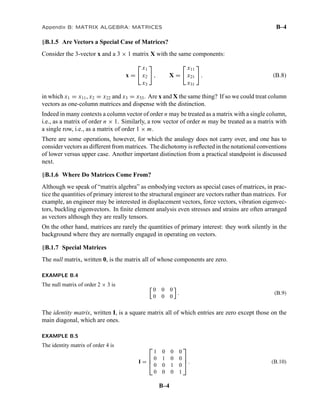
EXAMPLE B.2
12 6 3
C= 8 24 7 (B.5)
2 5 11
is a square matrix of order 3.
Consider a square matrix A = [ai j ] of order n × n. Its n components aii form the main diagonal,
which runs from top left to bottom right. The cross diagonal runs from the bottom left to upper
right. The main diagonal of the example matrix (B.5) is {12, 24, 11} and the cross diagonal is
{2, 24, 3}.
Entries that run parallel to and above (below) the main diagonal form superdiagonals (subdiagonals).
For example, {6, 7} is the first superdiagonal of the example matrix (B.5).
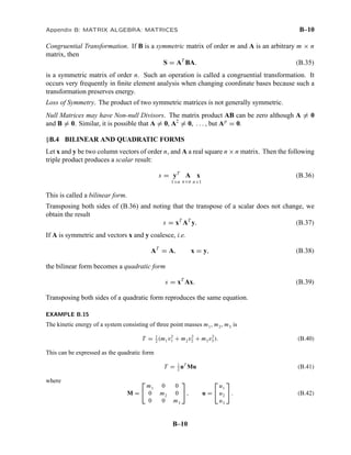
§B.1.4 Symmetry and Antisymmetry
Square matrices for which ai j = a ji are called symmetric about the main diagonal or simply
symmetric.
Square matrices for which ai j = −a ji are called antisymmetric or skew-symmetric. The diagonal
entries of an antisymmetric matrix must be zero.
EXAMPLE B.3
The following is a symmetric matrix of order 3:
11 6 1
S= 6 3 −1 . (B.6)
1 −1 −6
The following is an antisymmetric matrix of order 4:
 
0 3 −1 −5
 −3 0 7 −2 
W= . (B.7)
1 −7 0 0
5 2 0 0
B–3

4. Appendix B: MATRIX ALGEBRA: MATRICES B–4
§B.1.5 Are Vectors a Special Case of Matrices?
Consider the 3-vector x and a 3 × 1 matrix X with the same components:
x1 x11
x= x2 , X= x21 . (B.8)
x3 x31
in which x1 = x11 , x2 = x22 and x3 = x33 . Are x and X the same thing? If so we could treat column
vectors as one-column matrices and dispense with the distinction.
Indeed in many contexts a column vector of order n may be treated as a matrix with a single column,
i.e., as a matrix of order n × 1. Similarly, a row vector of order m may be treated as a matrix with
a single row, i.e., as a matrix of order 1 × m.
There are some operations, however, for which the analogy does not carry over, and one has to
consider vectors as different from matrices. The dichotomy is reflected in the notational conventions
of lower versus upper case. Another important distinction from a practical standpoint is discussed
next.
§B.1.6 Where Do Matrices Come From?
Although we speak of “matrix algebra” as embodying vectors as special cases of matrices, in prac-
tice the quantities of primary interest to the structural engineer are vectors rather than matrices. For
example, an engineer may be interested in displacement vectors, force vectors, vibration eigenvec-
tors, buckling eigenvectors. In finite element analysis even stresses and strains are often arranged
as vectors although they are really tensors.
On the other hand, matrices are rarely the quantities of primary interest: they work silently in the
background where they are normally engaged in operating on vectors.
§B.1.7 Special Matrices
The null matrix, written 0, is the matrix all of whose components are zero.
EXAMPLE B.4
The null matrix of order 2 × 3 is
0 0 0
. (B.9)
0 0 0
The identity matrix, written I, is a square matrix all of which entries are zero except those on the
main diagonal, which are ones.
EXAMPLE B.5
The identity matrix of order 4 is  
1 0 0 0
0 1 0 0
I= . (B.10)
0 0 1 0
0 0 0 1
B–4

5. B–5 §B.2 ELEMENTARY MATRIX OPERATIONS
A diagonal matrix is a square matrix all of which entries are zero except for those on the main
diagonal, which may be arbitrary.
EXAMPLE B.6
The following matrix of order 4 is diagonal:
 
14 0 0 0
 0 −6 0 0 
D= . (B.11)
0 0 0 0
0 0 0 3
A short hand notation which lists only the diagonal entries is sometimes used for diagonal matrices to save
writing space. This notation is illustrated for the above matrix:
D = diag [ 14 −6 0 3 ]. (B.12)
An upper triangular matrix is a square matrix in which all elements underneath the main diagonal
vanish. A lower triangular matrix is a square matrix in which all entries above the main diagonal
vanish.
EXAMPLE B.7
Here are examples of each kind:
   
6 4 2 1 5 0 0 0
0 6 4 2  10 4 0 0
U= , L= . (B.13)
0 0 6 4 −3 21 6 0
0 0 0 6 −15 −2 18 7
§B.2 ELEMENTARY MATRIX OPERATIONS
§B.2.1 Equality
Two matrices A and B of same order m × n are said to be equal if and only if all of their components
are equal: ai j = bi j , for all i = 1, . . . m, j = 1, . . . n. We then write A = B. If the inequality test
fails the matrices are said to be unequal and we write A = B.
Two matrices of different order cannot be compared for equality or inequality.
There is no simple test for greater-than or less-than.
§B.2.2 Transposition
The transpose of a matrix A is another matrix denoted by AT that has n rows and m columns
AT = [a ji ]. (B.14)
The rows of AT are the columns of A, and the rows of A are the columns of AT .
Obviously the transpose of AT is again A, that is, (AT )T = A.
B–5

6. Appendix B: MATRIX ALGEBRA: MATRICES B–6
EXAMPLE B.8
5 1
5 7 0
A= , AT = 7 0 . (B.15)
1 0 4
0 4
The transpose of a square matrix is also a square matrix. The transpose of a symmetric matrix A
is equal to the original matrix, i.e., A = AT . The negated transpose of an antisymmetric matrix
matrix A is equal to the original matrix, i.e. A = −AT .
EXAMPLE B.9
4 7 0 0 7 0
A= 7 1 2 = AT , W= −7 0 −2 = −WT (B.16)
0 2 3 0 2 0
§B.2.3 Addition and Subtraction
The simplest operation acting on two matrices is addition. The sum of two matrices of the same
order, A and B, is written A + B and defined to be the matrix
def
A + B = [ai j + bi j ]. (B.17)
Like vector addition, matrix addition is commutative: A+B = B+A, and associative: A+(B+C) =
(A + B) + C. For n = 1 or m = 1 the operation reduces to the addition of two column or row
vectors, respectively.
For matrix subtraction, replace + by − in the definition (B.17).
EXAMPLE B.10
The sum of
1 −3 0 6 3 −3 7 0 −3
A= and B= is A + B = . (B.18)
4 2 −1 7 −2 5 11 0 4
§B.2.4 Scalar Multiplication
Multiplication of a matrix A by a scalar c is defined by means of the relation
def
c A = [cai j ] (B.19)
That is, each entry of the matrix is multiplied by c. This operation is often called scaling of a matrix.
If c = 0, the result is the null matrix. Division of a matrix by a nonzero scalar c is equivalent to
multiplication by (1/c).
EXAMPLE B.11
1 −3 0 3 −9 0
If A= , 3A = . (B.20)
4 2 −1 12 6 −3
B–6

7. B–7 §B.3 MATRIX PRODUCTS
§B.3 MATRIX PRODUCTS
§B.3.1 Matrix by Vector
Before describing the general matrix product of two matrices, let us treat the particular case in
which the second matrix is a column vector. This so-called matrix-vector product merits special
attention because it occurs very frequently in the applications. Let A = [ai j ] be an m × n matrix,
x = {x j } a column vector of order n, and y = {yi } a column vector of order m. The matrix-vector
product is symbolically written
y = Ax, (B.21)
to mean the linear transformation
n
def sc
yi = ai j x j = ai j x j , i = 1, . . . , m. (B.22)
j=1
EXAMPLE B.12
The product of a 2 × 3 matrix and a vector of order 3 is a vector of order 2:
1
1 −3 0 −5
2 = (B.23)
4 2 −1 5
3
This product definition is not arbitrary but emanates from the analytical and geometric properties
of entities represented by matrices and vectors.
For the product definition to make sense, the column dimension of the matrix A (called the pre-
multiplicand) must equal the dimension of the vector x (called the post-multiplicand). For example,
the reverse product xA does not make sense unless m = n = 1.
If the row dimension m of A is one, the matrix formally reduces to a row vector (see §A.2), and the
matrix-vector product reduces to the inner product defined by Equation (A.11). The result of this
operation is a one-dimensional vector or scalar. We thus see that the present definition properly
embodies previous cases.
The associative and commutative properties of the matrix-vector product fall under the rules of the
more general matrix-matrix product discussed next.
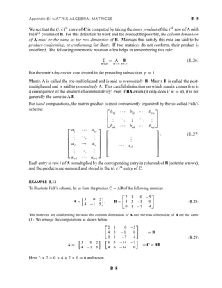
§B.3.2 Matrix by Matrix
We now pass to the most general matrix-by-matrix product, and consider the operations involved
in computing the product C of two matrices A and B:
C = AB. (B.24)
Here A = [ai j ] is a matrix of order m × n, B = [b jk ] is a matrix of order n × p, and C = [cik ] is a
matrix of order m × p. The entries of the result matrix C are defined by the formula
n
def sc
cik = ai j b jk = ai j b jk , i = 1, . . . , m, k = 1, . . . , p. (B.25)
j=1
B–7

8. Appendix B: MATRIX ALGEBRA: MATRICES B–8
We see that the (i, k)th entry of C is computed by taking the inner product of the i th row of A with
the k th column of B. For this definition to work and the product be possible, the column dimension
of A must be the same as the row dimension of B. Matrices that satisfy this rule are said to be
product-conforming, or conforming for short. If two matrices do not conform, their product is
undefined. The following mnemonic notation often helps in remembering this rule:
C = A B (B.26)
m× p m×n n× p
For the matrix-by-vector case treated in the preceding subsection, p = 1.
Matrix A is called the pre-multiplicand and is said to premultiply B. Matrix B is called the post-
multiplicand and is said to postmultiply A. This careful distinction on which matrix comes first is
a consequence of the absence of commutativity: even if BA exists (it only does if m = n), it is not
generally the same as AB.
For hand computations, the matrix product is most conveniently organized by the so-called Falk’s
scheme:  
b11 · · · bik · · · b1 p
 . .. .. . 
 . . . ↓ . . 
.
bn1 · · · bnk · · · bnp
a · · · a1n   
11
 . .. .  . (B.27)
 . . . .  
. 
.
.
.


 
 ai1 → ain    · · · cik


 . .   
 . .. .
. . .
am1 · · · amn
Each entry in row i of A is multiplied by the corresponding entry in column k of B (note the arrows),
and the products are summed and stored in the (i, k)th entry of C.
EXAMPLE B.13
To illustrate Falk’s scheme, let us form the product C = AB of the following matrices
2 1 0 −5
3 0 2
A= , B= 4 3 −1 0 (B.28)
4 −1 5
0 1 −7 4
The matrices are conforming because the column dimension of A and the row dimension of B are the same
(3). We arrange the computations as shown below:
2 1 0 −5
4 3 −1 0 =B
0 1 −7 4 (B.29)
3 0 2 6 5 −14 −7
A= = C = AB
4 −1 5 4 6 −34 0
Here 3 × 2 + 0 × 4 + 2 × 0 = 6 and so on.
B–8

9. B–9 §B.3 MATRIX PRODUCTS
§B.3.3 Matrix Powers
If A = B, the product AA is called the square of A and is denoted by A2 . Note that for this definition
to make sense, A must be a square matrix.
Similarly, A3 = AAA = A2 A = AA2 . Other positive-integer powers can be defined in an
analogous manner.
This definition does not encompass negative powers. For example, A−1 denotes the inverse of matrix
A, which is studied in Appendix C. The general power Am , where m can be a real or complex scalar,
can be defined with the help of the matrix spectral form and require the notion of eigensystem.
A square matrix A that satisfies A = A2 is called idempotent. We shall see later that that equation
characterizes the so-called projector matrices.
A square matrix A whose p th power is the null matrix is called p-nilpotent.
§B.3.4 Properties of Matrix Products
Associativity. The associative law is verified:
A(BC) = (AB)C. (B.30)
Hence we may delete the parentheses and simply write ABC.
Distributivity. The distributive law also holds: If B and C are matrices of the same order, then
A (B + C) = AB + AC, and (B + C) A = BA + CA. (B.31)
Commutativity. The commutativity law of scalar multiplication does not generally hold. If A and
B are square matrices of the same order, then the products AB and BA are both possible but in
general AB = BA.
If AB = BA, the matrices A and B are said to commute. One important case is when A and B are
diagonal. In general A and B commute if they share the same eigensystem.
EXAMPLE B.14
Matrices
a b a−β b
A= , B= , (B.32)
b c b c−β
commute for any a, b, c, β. More generally, A and B = A − βI commute for any square matrix A.
Transpose of a Product. The transpose of a matrix product is equal to the product of the transposes
of the operands taken in reverse order:
(AB)T = BT AT . (B.33)
The general transposition formula for an arbitrary product sequence is
(ABC . . . MN)T = NT MT . . . CT BT AT . (B.34)
B–9

10. Appendix B: MATRIX ALGEBRA: MATRICES B–10
Congruential Transformation. If B is a symmetric matrix of order m and A is an arbitrary m × n
matrix, then
S = AT BA. (B.35)
is a symmetric matrix of order n. Such an operation is called a congruential transformation. It
occurs very frequently in finite element analysis when changing coordinate bases because such a
transformation preserves energy.
Loss of Symmetry. The product of two symmetric matrices is not generally symmetric.
Null Matrices may have Non-null Divisors. The matrix product AB can be zero although A = 0
and B = 0. Similar, it is possible that A = 0, A2 = 0, . . . , but A p = 0.
§B.4 BILINEAR AND QUADRATIC FORMS
Let x and y be two column vectors of order n, and A a real square n × n matrix. Then the following
triple product produces a scalar result:
s = yT A x (B.36)
1×n n×n n×1
This is called a bilinear form.
Transposing both sides of (B.36) and noting that the transpose of a scalar does not change, we
obtain the result
s = xT AT y. (B.37)
If A is symmetric and vectors x and y coalesce, i.e.
AT = A, x = y, (B.38)
the bilinear form becomes a quadratic form
s = xT Ax. (B.39)
Transposing both sides of a quadratic form reproduces the same equation.
EXAMPLE B.15
The kinetic energy of a system consisting of three point masses m 1 , m 2 , m 3 is
T = 1 (m 1 v1 + m 2 v2 + m 3 v3 ).
2
2 2 2
(B.40)
This can be expressed as the quadratic form
T = 1 uT Mu
2
(B.41)
where
m1 0 0 u1
M= 0 m2 0 , u= u2 . (B.42)
0 0 m3 u3
B–10

11. B–11 Exercises
Homework Exercises for Appendix B: Matrices
EXERCISE B.1
Given the three matrices
 
2 −2
2 4 1 0
 1 0 1 −3 2
A= −1 , B= , C= (EB.1)
1
2 3 1
4 2 0 2
2 5 −1 2
−3 2
compute the product D = ABC by hand using Falk’s scheme. (Hint: do BC first, then premultiply that by
A.)
EXERCISE B.2
Given the square matrices
1 3 3 0
A= , B= (EB.2)
−4 2 1 −2
verify by direct computation that AB = BA.
EXERCISE B.3
Given the matrices
1 0 3 −1 4
A= −1 2 , B= −1 2 0 (EB.3)
2 0 4 0 0
(note that B is symmetric) compute S = AT BA, and verify that S is symmetric.
EXERCISE B.4
Given the square matrices
3 −1 2 3 −6 −3
A= 1 0 3 , B= 7 −14 −7 (EB.4)
3 −2 −5 −1 2 1
verify that AB = 0 although A = 0 and B = 0. Is BA also null?
EXERCISE B.5
Given the square matrix
0 a b
A= 0 0 c (EB.5)
0 0 0
show by direct computation that A2 = 0 but A3 = 0.
EXERCISE B.6
Can a diagonal matrix be antisymmetric?
B–11

12. Appendix B: MATRIX ALGEBRA: MATRICES B–12
EXERCISE B.7
(Tougher) Prove (B.33). (Hint: call C = (AB)T , D = BT AT , and use the matrix product definition (B.25) to
show that the generic entries of C and D agree.)
EXERCISE B.8
If A is an arbitrary m × n matrix, show: (a) both products AT A and AAT are possible, and (b) both products
are square and symmetric. (Hint: for (b) make use of the symmetry condition S = ST and of (B.31).)
EXERCISE B.9
Show that A2 only exists if and only if A is square.
EXERCISE B.10
If A is square and antisymmetric, show that A2 is symmetric. (Hint: start from A = −AT and apply the results
of Exercise B.8.)
B–12

13. B–13 Solutions to Exercises
Homework Exercises for Appendix B - Solutions
EXERCISE B.1
1 −3 2
=C
   2 0 2 
2 −2 −2 −6 0
 1 0  1 −3 2
B=   6 −12 10  = BC
4 1
−3 2 1 9 −2
2 4 1 0 6 −36 18
A= −1 2 3 1 23 −27 32 = ABC = D
2 5 −1 2 −3 3 −4
EXERCISE B.2
6 −6 3 9
AB = = BA =
−10 −4 9 −1
EXERCISE B.3
23 −6
S = AT BA =
−6 8
which is symmetric, like B.
EXERCISE B.4
3 −6 −3
7 −14 −7 = B
−1 2 1
3 −1 2 0 0 0
A= 1 0 3 0 0 0 = AB = 0
3 −2 −5 0 0 0
However,
−6 3 3
BA = −14 7 7 =0
2 −1 −1
EXERCISE B.5
0 0 ac 0 0 0
A2 = AA = 0 0 0 , A3 = AAA = 0 0 0 =0
0 0 0 0 0 0
EXERCISE B.6
Only if it is the null matrix.
B–13

14. Appendix B: MATRIX ALGEBRA: MATRICES B–14
EXERCISE B.7
To avoid “indexing indigestion” let us carefully specify the dimensions of the given matrices and their trans-
poses:
A = [ai j ], AT = [a ji ]
m×n n×m
B = [b jk ], BT = [bk j ]
n× p p×n
Indices i, j and k run over 1 . . . m, 1 . . . n and 1 . . . p, respectively. Now call
C = [cki ] = (AB)T
p×m
D = [dki ] = BT AT
p×m
From the definition of matrix product,
n
cki = ai j b jk
j=1
n n
dki = b jk ai j = ai j b jk = cki
j=1 j=1
hence C = D for any A and B, and the statement is proved.
EXERCISE B.8
(a) If A is m × n, AT is n × m. Next we write the two products to be investigated:
AT A , A AT
n×m m×n m×n n×m
In both cases the column dimension of the premultiplicand is equal to the row dimension of the postmultiplicand.
Therefore both products are possible.
(b) To verify symmetry we use three results. First, the symmetry test: transpose equals original; second,
transposing twice gives back the original; and, finally, the transposed-product formula proved in Exercise B.7.
(AT A)T = AT (AT )T = AT A
(AAT )T = (AT )T AT = AAT
Or, to do it more slowly, call B = AT , BT = A, C = AB, and let’s go over the first one again:
CT = (AB)T = BT AT = AAT = AB = C
Since C = CT , C = AAT is symmetric. Same mechanics for the second one.
EXERCISE B.9
Let A be m × n. For A2 = AA to exist, the column dimension n of the premultiplicand A must equal the row
dimension m of the postmultiplicand A. Hence m = n and A must be square.
EXERCISE B.10
Premultiply both sides of A = −AT by A (which is always possible because A is square):
A2 = AA = −AAT
But from Exercise B.8 we know that AAT is symmetric. Since the negated of a symmetric matrix is symmetric,
so is A2 .
B–14