Download as PDF, PPTX


![introduction: data streams
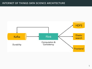
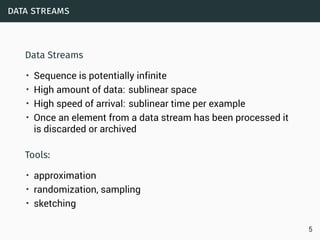
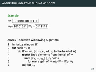
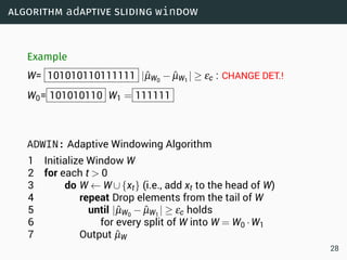
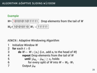
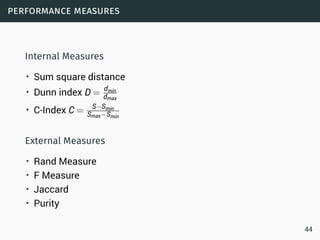
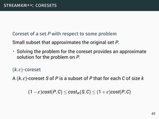
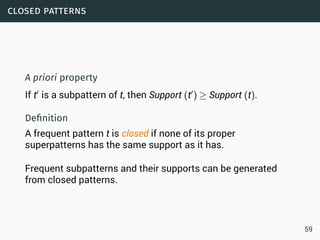
Data Streams
• Sequence is potentially infinite
• High amount of data: sublinear space
• High speed of arrival: sublinear time per example
• Once an element from a data stream has been processed it
is discarded or archived
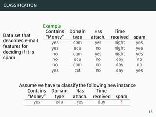
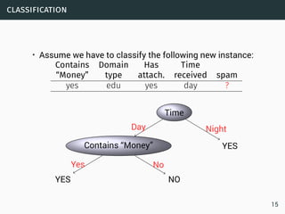
Example
Puzzle: Finding Missing Numbers
• Let π be a permutation of {1,...,n}.
• Let π−1 be π with one element missing.
• π−1[i] arrives in increasing order
Task: Determine the missing number
4](https://image.slidesharecdn.com/bigdata-streammining-151217230150/85/Internet-of-Things-Data-Science-5-320.jpg)
![introduction: data streams
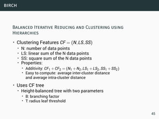
Data Streams
• Sequence is potentially infinite
• High amount of data: sublinear space
• High speed of arrival: sublinear time per example
• Once an element from a data stream has been processed it
is discarded or archived
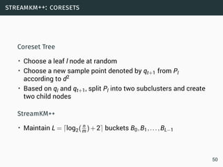
Example
Puzzle: Finding Missing Numbers
• Let π be a permutation of {1,...,n}.
• Let π−1 be π with one element missing.
• π−1[i] arrives in increasing order
Task: Determine the missing number
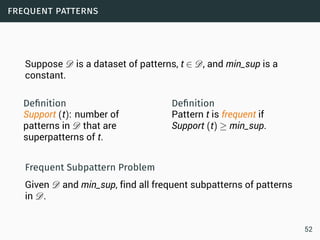
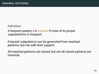
Use a n-bit
vector to
memorize all the
numbers (O(n)
space)
4](https://image.slidesharecdn.com/bigdata-streammining-151217230150/85/Internet-of-Things-Data-Science-6-320.jpg)
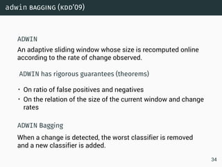
![introduction: data streams
Data Streams
• Sequence is potentially infinite
• High amount of data: sublinear space
• High speed of arrival: sublinear time per example
• Once an element from a data stream has been processed it
is discarded or archived
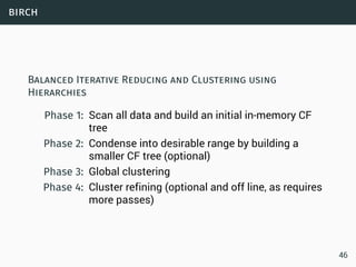
Example
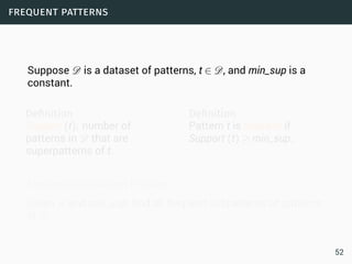
Puzzle: Finding Missing Numbers
• Let π be a permutation of {1,...,n}.
• Let π−1 be π with one element missing.
• π−1[i] arrives in increasing order
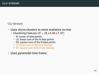
Task: Determine the missing number
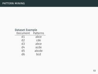
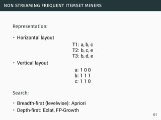
Data Streams:
O(log(n)) space.
4](https://image.slidesharecdn.com/bigdata-streammining-151217230150/85/Internet-of-Things-Data-Science-7-320.jpg)
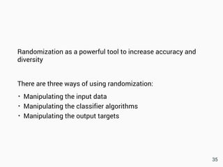
![introduction: data streams
Data Streams
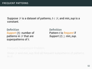
• Sequence is potentially infinite
• High amount of data: sublinear space
• High speed of arrival: sublinear time per example
• Once an element from a data stream has been processed it
is discarded or archived
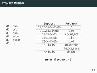
Example
Puzzle: Finding Missing Numbers
• Let π be a permutation of {1,...,n}.
• Let π−1 be π with one element missing.
• π−1[i] arrives in increasing order
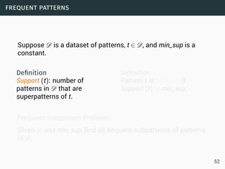
Task: Determine the missing number
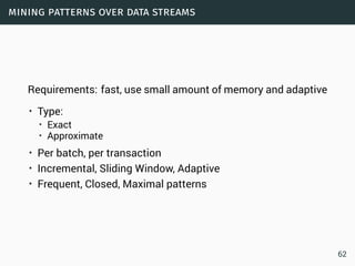
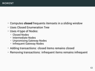
Data Streams:
O(log(n)) space.
Store
n(n+1)
2
−∑
j≤i
π−1[j].
4](https://image.slidesharecdn.com/bigdata-streammining-151217230150/85/Internet-of-Things-Data-Science-8-320.jpg)
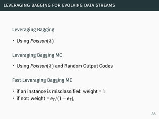
![data streams
Data Streams
• Sequence is potentially infinite
• High amount of data: sublinear space
• High speed of arrival: sublinear time per example
• Once an element from a data stream has been processed it
is discarded or archived
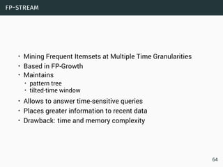
Approximation algorithms
• Small error rate with high probability
• An algorithm (ε,δ)−approximates F if it outputs ˜F for which
Pr[|˜F−F| > εF] < δ.
5](https://image.slidesharecdn.com/bigdata-streammining-151217230150/85/Internet-of-Things-Data-Science-10-320.jpg)


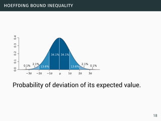
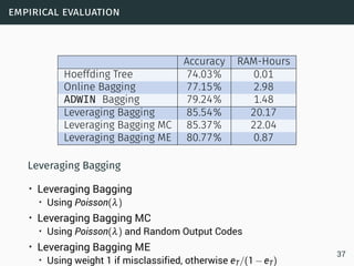
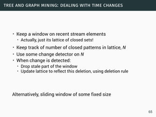
![hoeffding bound inequality
Let X = ∑i Xi where X1,...,Xn are independent and indentically
distributed in [0,1]. Then
1 Chernoff For each ε < 1
Pr[X > (1+ε)E[X]] ≤ exp
(
−
ε2
3
E[X]
)
2 Hoeffding For each t > 0
Pr[X > E[X]+t] ≤ exp
(
−2t2
/n
)
3 Bernstein Let σ2 = ∑i σ2
i the variance of X. If Xi −E[Xi] ≤ b for
each i ∈ [n] then for each t > 0
Pr[X > E[X]+t] ≤ exp
(
−
t2
2σ2 + 2
3bt
)
19](https://image.slidesharecdn.com/bigdata-streammining-151217230150/85/Internet-of-Things-Data-Science-32-320.jpg)
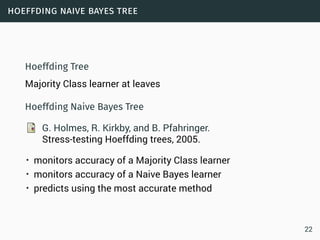

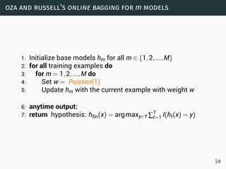

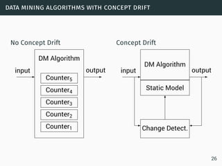
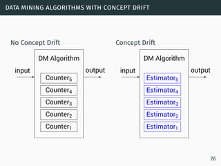
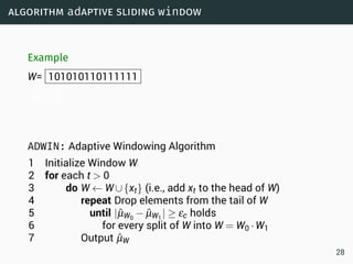
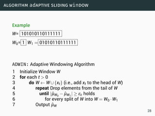


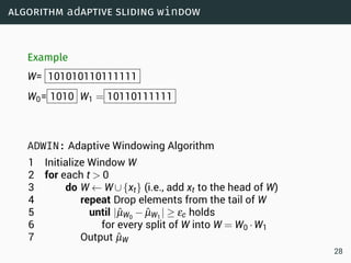
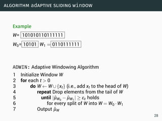


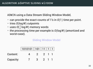
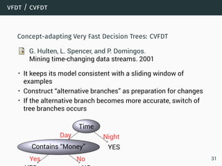
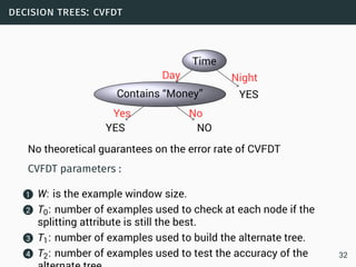
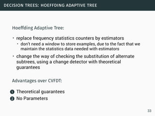


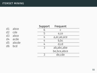
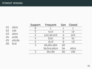

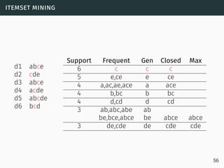
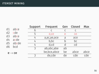


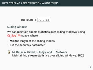
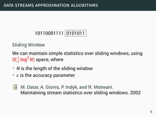
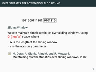
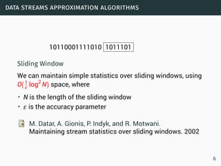
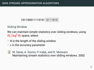
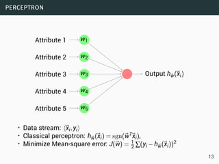
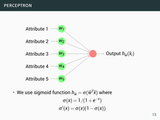
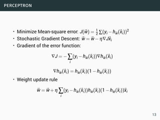
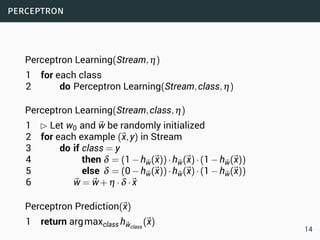
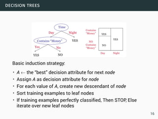
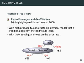
The document discusses data stream classification and algorithms for handling data streams. It begins with an introduction to data stream characteristics and challenges. It then discusses approximation algorithms for data streams, including maintaining statistics over sliding windows. Classification algorithms for data streams discussed include Naive Bayes classifiers, perceptrons, and Hoeffding trees, which are decision trees adapted for data streams using the Hoeffding bound inequality to determine the optimal split attribute.