Data streaming algorithms
Sandeep Joshi
Chief hacker
1
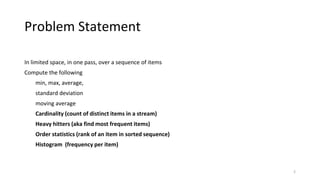
Problem Statement
In limited space, in one pass, over a sequence of items
Compute the following
min, max, average,
standard deviation
moving average
Cardinality (count of distinct items in a stream)
Heavy hitters (aka find most frequent items)
Order statistics (rank of an item in sorted sequence)
Histogram (frequency per item)
2
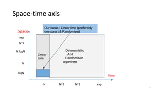
Space-time axis
3
Space
Time
N N^2 N^3 exp
N
N.logN
logN
N^k
Deterministic
And
Randomized
algorithms
Linear
time
Our focus : Linear time (preferably
one pass) & Randomized
exp
Approach
• Will present simplified algorithms to provide general idea.
• Not going to cover all proposed solutions for a problem.
• Sacrifice rigor to provide intuition.
4
Not going to cover
• Sampling techniques
• Case where input is sequence of strings or multi-dimensional
• Set membership problem (bloom filters, etc)
• Outlier detection
• Time series-related algorithms
• How to extend algorithms to distributed setting
5
1. Cardinality
6
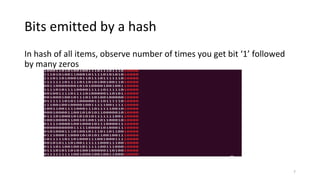
Bits emitted by a hash
In hash of all items, observe number of times you get bit ‘1’ followed
by many zeros
7
Bit patterns
For num = [1, 1000]
h = hash(num)
Number of hashes ending in Out of 1000
0 530
10 281
100 140
1000 53
10000 28
100000 9
1000000 12
10000000 5
100000000 2
1000000000 0
10000000000 0
100000000000 0
8
Bit ‘1’ followed by 9 or
more zeroes not found
Because 1000 ~ 2^10
Flajolet-Martin sketch algo
1. For each item
2. Index = rightmost bit in hash(item)
3. Bitmap[index] = 1
(at this point, bitmap = “000...00000101011111”)
1. Estimated N ~ 2 rightmost ‘0’ bit in bitmap
9
Further improvements : split stream into M substreams and use harmonic mean of their
counters, use 64-bit hash instead of 32, add custom correction factors to hash at low and high
range.
Why it works
• The number of distinct items can be roughly estimated by the
position of the rightmost 0-bit.
• A randomized algorithm which takes sublinear space - number of bits
is equal to log2(n)
• Algorithm also works over strings [ 1985 paper uses strings ]
• Any set of bits can be used [ hyperloglog uses middle bits]
10
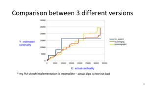
Comparison between 3 different versions
* my FM-sketch implementation is incomplete – actual algo is not that bad
11
X : actual cardinality
Y : estimated
cardinality
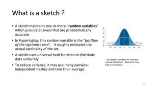
What is a sketch ?
• A sketch maintains one or more “random variables”
which provide answers that are probabilistically
accurate.
• In Hyperloglog, this random variable is the “position
of the rightmost zero”. It roughly estimates the
actual cardinality of the set.
• A sketch uses universal hash function to distribute
data uniformly.
• To reduce variance, it may use many pairwise-
independent hashes and take their average.
12
* all random variables do not have
normal distribution. Above Pic is to
help in visualizing
2. Heavy Hitters
13
Heavy Hitters problem
• Find the items in a sequence which occur most frequently
• We will see two algorithms
1. Karp, Shenker and Papadimitrou
2. Count-Min sketch by Cormode and Muthukrishnan. Versatile algo
which has many applications
14
Heavy Hitters – Karp, et al
1. Keep a frequency Map<item, count>
2. For each v in sequence
3. increment Map[v].count
4. If map.size() > threshold
5. for each element in Map
6. decrement Map[element].count
7. if count is zero, delete Map[element]
Algo has second pass to adjust counts. Paper discusses additional optimizations.
Implemented in Apache Spark. See DataFrameStatFunctions.freqItems().
Maintain a truncated histogram
15
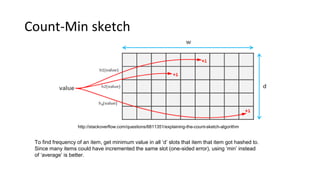
Count-Min sketch
http://stackoverflow.com/questions/6811351/explaining-the-count-sketch-algorithm
To find frequency of an item, get minimum value in all ‘d’ slots that item that item got hashed to.
Since many items could have incremented the same slot (one-sided error), using ‘min’ instead
of ‘average’ is better.
Count-Min Sketch applications
• For heavy hitters, need additional heap data structure to maintain
those items which hashed to high value slots.
• Point query
• Range query using dyadic ranges
• Joins
• Temporal extension (Hokusai) to store historical sketches at lower
resolution.
17
3.Order statistics
18
Order statistics terminology
Given sorted sequence [1, 1, 1, 2, 3]
1. 0-quantile = minimum
2. 0.25 quantile = 1st quartile = 25 percentile
3. 0.50 quantile = 2nd quartile = 50 percentile = median
4. 0.75 quantile = 3rd quartile = 75 percentile
5. 1-quantile = maximum
19
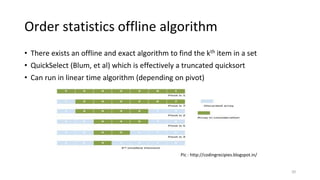
Order statistics offline algorithm
• There exists an offline and exact algorithm to find the kth item in a set
• QuickSelect (Blum, et al) which is effectively a truncated quicksort
• Can run in linear time algorithm (depending on pivot)
20
Pic : http://codingrecipies.blogspot.in/
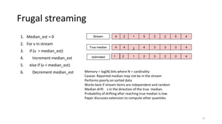
Frugal streaming
1. Median_est = 0
2. For v in stream
3. if (v > median_est)
4. Increment median_est
5. else if (v < median_est)
6. Decrement median_est
21
Memory = log(N) bits where N = cardinality
Caveat: Reported median may not be in the stream
Performs poorly on sorted data
Works best if stream items are independent and random
Median drift s in the direction of the true median.
Probability of drifting after reaching true median is low.
Paper discusses extension to compute other quantiles
4 2 1 5 52 43
4 4 2 4 33 43
2 1 2 32 43
Stream
True median
estimated 1
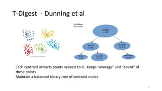
T-Digest - Dunning et al
22
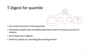
Each centroid attracts points nearest to it. Keeps “average” and “count” of
these points.
Maintain a balanced binary tree of centroid nodes
T-Digest for quantile
• Use sorted structure to find quantiles.
• Centroids at both ends are deliberately kept small to increase accuracy of
outliers.
• Can merge two T-digests.
• Performs poorly on ascending/descending stream.
23
4. Histogram
24
Histogram
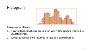
Two major problems
1. How to decide bucket ranges apriori when data is being inserted in
unsorted order.
2. What count should be returned in case of a partial bucket.
25
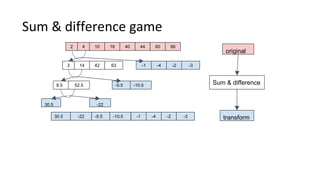
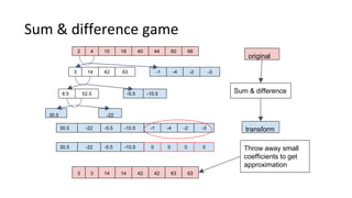
Sum & difference game
2 4 10 18 6044 6640
3 14 42 63 -1 -4 -2 -3
8.5 52.5 -5.5 -10.5
30.5 -22
30.5 -22 -5.5 -10.5 -1 -4 -2 -3
original
transform
Sum & difference
Sum & difference game
2 4 10 18 6044 6640
3 14 42 63 -1 -4 -2 -3
8.5 52.5 -5.5 -10.5
30.5 -22
30.5 -22 -5.5 -10.5 -1 -4 -2 -3
original
transform
Sum & difference
3 3 14 14 6342 6342
30.5 -22 -5.5 -10.5 0 0 0 0 Throw away small
coefficients to get
approximation
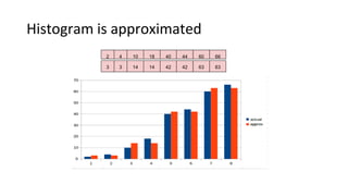
Histogram is approximated
2 4 10 18 6044 6640
3 3 14 14 6342 6342
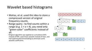
Wavelet based histograms
• Matias, et al. used this idea to store a
compressed version of original
frequency counts.
• Range query : to find counts within a
range (e.g. 1 < x < 4), you need only
“green-color” coefficients instead of
all.
•Original algorithm was applied on cumulative (CDF)
instead of PDF; used linear wavelet instead of Haar, and
had sophisticated thresholding to eliminate some
wavelet coefficients.
29
2 4 10 18 6044 6640
3 14 42 63 -1 -4 -2 -3
8.5 52.5 -5.5 -10.5
30.5 -22
30.5 -22 -5.5 -10.5 -1 -4 -2 -3
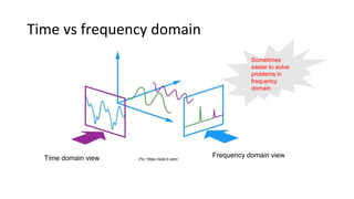
Time vs frequency domain
Time domain view Frequency domain viewPic; https://e2e.ti.com/
Sometimes
easier to solve
problems in
frequency
domain
References
• Blog : https://research.neustar.biz/tag/streaming-algorithms/
• Code : http://github.com/clearspring/stream-lib
• Code : http://github.com/twitter/algebird
• Book : Ullman et al, Mining Massive Data sets
• Gist : http://gist.github.com/debasishg/8172796
31
Backup
K-min values for cardinality
Munro-Paterson : median cannot be calculated exactly without O(n)
memory. Similar result for cardinality and heavy-hitters.
Wavelet : transform takes O(N), thresholding takes O(N.logN.logm),
query takes O(m) where m = truncated coeff, N = original data.
Histogram from various perspectives
• Statistics : known as “density estimation”. Its non-parametric
because we are not told how points are distributed ahead of time.
Two approaches
1) parzen windows
2) nearest neighbour (k-means).
• Computer science : k-segmentation problem; solved with Bellman’s
dynamic programming algorithm.
• Signal processing : translate time domain problem into frequency
domain.
33

Data streaming algorithms

  • 1.
  • 2.
    Problem Statement In limitedspace, in one pass, over a sequence of items Compute the following min, max, average, standard deviation moving average Cardinality (count of distinct items in a stream) Heavy hitters (aka find most frequent items) Order statistics (rank of an item in sorted sequence) Histogram (frequency per item) 2
  • 3.
    Space-time axis 3 Space Time N N^2N^3 exp N N.logN logN N^k Deterministic And Randomized algorithms Linear time Our focus : Linear time (preferably one pass) & Randomized exp
  • 4.
    Approach • Will presentsimplified algorithms to provide general idea. • Not going to cover all proposed solutions for a problem. • Sacrifice rigor to provide intuition. 4
  • 5.
    Not going tocover • Sampling techniques • Case where input is sequence of strings or multi-dimensional • Set membership problem (bloom filters, etc) • Outlier detection • Time series-related algorithms • How to extend algorithms to distributed setting 5
  • 6.
  • 7.
    Bits emitted bya hash In hash of all items, observe number of times you get bit ‘1’ followed by many zeros 7
  • 8.
    Bit patterns For num= [1, 1000] h = hash(num) Number of hashes ending in Out of 1000 0 530 10 281 100 140 1000 53 10000 28 100000 9 1000000 12 10000000 5 100000000 2 1000000000 0 10000000000 0 100000000000 0 8 Bit ‘1’ followed by 9 or more zeroes not found Because 1000 ~ 2^10
  • 9.
    Flajolet-Martin sketch algo 1.For each item 2. Index = rightmost bit in hash(item) 3. Bitmap[index] = 1 (at this point, bitmap = “000...00000101011111”) 1. Estimated N ~ 2 rightmost ‘0’ bit in bitmap 9 Further improvements : split stream into M substreams and use harmonic mean of their counters, use 64-bit hash instead of 32, add custom correction factors to hash at low and high range.
  • 10.
    Why it works •The number of distinct items can be roughly estimated by the position of the rightmost 0-bit. • A randomized algorithm which takes sublinear space - number of bits is equal to log2(n) • Algorithm also works over strings [ 1985 paper uses strings ] • Any set of bits can be used [ hyperloglog uses middle bits] 10
  • 11.
    Comparison between 3different versions * my FM-sketch implementation is incomplete – actual algo is not that bad 11 X : actual cardinality Y : estimated cardinality
  • 12.
    What is asketch ? • A sketch maintains one or more “random variables” which provide answers that are probabilistically accurate. • In Hyperloglog, this random variable is the “position of the rightmost zero”. It roughly estimates the actual cardinality of the set. • A sketch uses universal hash function to distribute data uniformly. • To reduce variance, it may use many pairwise- independent hashes and take their average. 12 * all random variables do not have normal distribution. Above Pic is to help in visualizing
  • 13.
  • 14.
    Heavy Hitters problem •Find the items in a sequence which occur most frequently • We will see two algorithms 1. Karp, Shenker and Papadimitrou 2. Count-Min sketch by Cormode and Muthukrishnan. Versatile algo which has many applications 14
  • 15.
    Heavy Hitters –Karp, et al 1. Keep a frequency Map<item, count> 2. For each v in sequence 3. increment Map[v].count 4. If map.size() > threshold 5. for each element in Map 6. decrement Map[element].count 7. if count is zero, delete Map[element] Algo has second pass to adjust counts. Paper discusses additional optimizations. Implemented in Apache Spark. See DataFrameStatFunctions.freqItems(). Maintain a truncated histogram 15
  • 16.
    Count-Min sketch http://stackoverflow.com/questions/6811351/explaining-the-count-sketch-algorithm To findfrequency of an item, get minimum value in all ‘d’ slots that item that item got hashed to. Since many items could have incremented the same slot (one-sided error), using ‘min’ instead of ‘average’ is better.
  • 17.
    Count-Min Sketch applications •For heavy hitters, need additional heap data structure to maintain those items which hashed to high value slots. • Point query • Range query using dyadic ranges • Joins • Temporal extension (Hokusai) to store historical sketches at lower resolution. 17
  • 18.
  • 19.
    Order statistics terminology Givensorted sequence [1, 1, 1, 2, 3] 1. 0-quantile = minimum 2. 0.25 quantile = 1st quartile = 25 percentile 3. 0.50 quantile = 2nd quartile = 50 percentile = median 4. 0.75 quantile = 3rd quartile = 75 percentile 5. 1-quantile = maximum 19
  • 20.
    Order statistics offlinealgorithm • There exists an offline and exact algorithm to find the kth item in a set • QuickSelect (Blum, et al) which is effectively a truncated quicksort • Can run in linear time algorithm (depending on pivot) 20 Pic : http://codingrecipies.blogspot.in/
  • 21.
    Frugal streaming 1. Median_est= 0 2. For v in stream 3. if (v > median_est) 4. Increment median_est 5. else if (v < median_est) 6. Decrement median_est 21 Memory = log(N) bits where N = cardinality Caveat: Reported median may not be in the stream Performs poorly on sorted data Works best if stream items are independent and random Median drift s in the direction of the true median. Probability of drifting after reaching true median is low. Paper discusses extension to compute other quantiles 4 2 1 5 52 43 4 4 2 4 33 43 2 1 2 32 43 Stream True median estimated 1
  • 22.
    T-Digest - Dunninget al 22 Each centroid attracts points nearest to it. Keeps “average” and “count” of these points. Maintain a balanced binary tree of centroid nodes
  • 23.
    T-Digest for quantile •Use sorted structure to find quantiles. • Centroids at both ends are deliberately kept small to increase accuracy of outliers. • Can merge two T-digests. • Performs poorly on ascending/descending stream. 23
  • 24.
  • 25.
    Histogram Two major problems 1.How to decide bucket ranges apriori when data is being inserted in unsorted order. 2. What count should be returned in case of a partial bucket. 25
  • 26.
    Sum & differencegame 2 4 10 18 6044 6640 3 14 42 63 -1 -4 -2 -3 8.5 52.5 -5.5 -10.5 30.5 -22 30.5 -22 -5.5 -10.5 -1 -4 -2 -3 original transform Sum & difference
  • 27.
    Sum & differencegame 2 4 10 18 6044 6640 3 14 42 63 -1 -4 -2 -3 8.5 52.5 -5.5 -10.5 30.5 -22 30.5 -22 -5.5 -10.5 -1 -4 -2 -3 original transform Sum & difference 3 3 14 14 6342 6342 30.5 -22 -5.5 -10.5 0 0 0 0 Throw away small coefficients to get approximation
  • 28.
    Histogram is approximated 24 10 18 6044 6640 3 3 14 14 6342 6342
  • 29.
    Wavelet based histograms •Matias, et al. used this idea to store a compressed version of original frequency counts. • Range query : to find counts within a range (e.g. 1 < x < 4), you need only “green-color” coefficients instead of all. •Original algorithm was applied on cumulative (CDF) instead of PDF; used linear wavelet instead of Haar, and had sophisticated thresholding to eliminate some wavelet coefficients. 29 2 4 10 18 6044 6640 3 14 42 63 -1 -4 -2 -3 8.5 52.5 -5.5 -10.5 30.5 -22 30.5 -22 -5.5 -10.5 -1 -4 -2 -3
  • 30.
    Time vs frequencydomain Time domain view Frequency domain viewPic; https://e2e.ti.com/ Sometimes easier to solve problems in frequency domain
  • 31.
    References • Blog :https://research.neustar.biz/tag/streaming-algorithms/ • Code : http://github.com/clearspring/stream-lib • Code : http://github.com/twitter/algebird • Book : Ullman et al, Mining Massive Data sets • Gist : http://gist.github.com/debasishg/8172796 31
  • 32.
    Backup K-min values forcardinality Munro-Paterson : median cannot be calculated exactly without O(n) memory. Similar result for cardinality and heavy-hitters. Wavelet : transform takes O(N), thresholding takes O(N.logN.logm), query takes O(m) where m = truncated coeff, N = original data.
  • 33.
    Histogram from variousperspectives • Statistics : known as “density estimation”. Its non-parametric because we are not told how points are distributed ahead of time. Two approaches 1) parzen windows 2) nearest neighbour (k-means). • Computer science : k-segmentation problem; solved with Bellman’s dynamic programming algorithm. • Signal processing : translate time domain problem into frequency domain. 33