Downloaded 20 times


![boosting
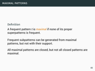
A formal description of Boosting (Schapire)
• given a training set (x1,y1),...,(xm,ym)
• yi ∈ {−1,+1} correct label of instance xi ∈ X
• for t = 1,...,T
• construct distribution Dt
• find weak classifier
ht : X → {−1,+1}
with small error εt = PrDt
[ht(xi) ̸= yi] on Dt
• output final classifier
17](https://image.slidesharecdn.com/bigdata-datascience-151217230811/85/Introduction-to-Big-Data-Science-21-320.jpg)


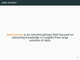
Data science involves extracting insights from large volumes of data. It is an interdisciplinary field that uses techniques from statistics, machine learning, and other domains. The document provides examples of classification algorithms like k-nearest neighbors, naive Bayes, and perceptrons that are commonly used in data science to build models for tasks like spam filtering or sentiment analysis. It also discusses clustering, frequent pattern mining, and other machine learning concepts.


![[ppt]](https://cdn.slidesharecdn.com/ss_thumbnails/ppt2931-thumbnail.jpg?width=640&height=640&fit=bounds)
![[ppt]](https://cdn.slidesharecdn.com/ss_thumbnails/ppt3441-thumbnail.jpg?width=640&height=640&fit=bounds)