
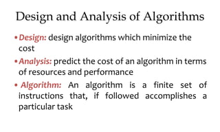
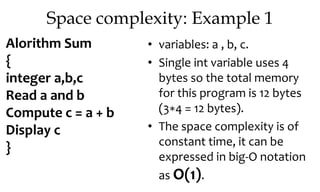
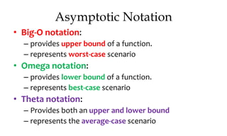
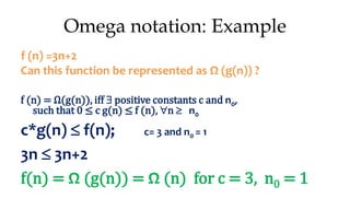
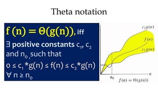
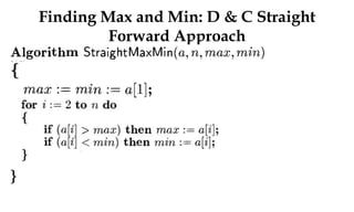
![Space complexity: Example 2
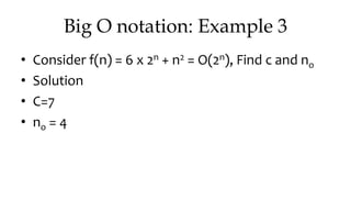
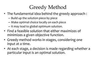
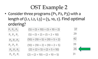
• Variables A[ ] is integer type with
size n so its space complexity is
4∗n bytes.
• Variables : n , i, arr_sum will take
4 bytes each, total 12 bytes
( 4∗3=12 bytes).
• Total memory this program
takes (4∗n+12) bytes.
• The space complexity is
increasing linearly with the size
n, it can be expressed in big-O
notation as O(n).
Procedure sum(A,n)
integer arr_sum
arr_sum 0
for i 0 to n do
arr_sum = arr_sum + A[i]
repeat
End sum](https://image.slidesharecdn.com/daapost-240405134921-2dcf40bc/85/Design-and-Analysis-of-Algorithms-Lecture-Notes-11-320.jpg)


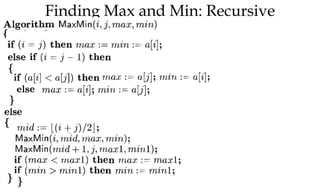
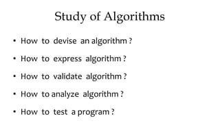
![Algorithm Merge(lb,mid,ub)
{
b: Auxiliary Array
i=lb;
j=mid+1;
k=lb;
while(i<=mid AND j<=ub)
{
if(a[i]<a[j]) b[k++]=a[i++];
else b[k++]=a[j++];
}
while(i<=mid) b[k++]=a[i++];
while(j<=ub) b[k++]=a[j++];
for(i=lb;i<=ub;i++) a[i]=b[i];
}](https://image.slidesharecdn.com/daapost-240405134921-2dcf40bc/85/Design-and-Analysis-of-Algorithms-Lecture-Notes-53-320.jpg)

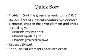

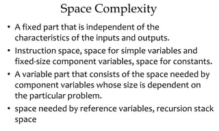
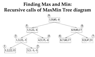
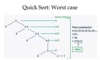
![Quick Sort
Algorithm partition(a,low,high)
{
}
pivot = a[high]; l = low; r = high - 1;
while (l < r)
{
while (a[l] <= pivot && l < r) l++;
while (a[r] >= pivot && l < r) r--;
swap(a, l, r);
}
if(a[l] > a[high]) swap(a,l,high);
else l = high;
return l;
Algorithm swap(a,i,j)
{
temp = a[i];
a[i] = a[j];
a[j] = temp;
}](https://image.slidesharecdn.com/daapost-240405134921-2dcf40bc/85/Design-and-Analysis-of-Algorithms-Lecture-Notes-61-320.jpg)
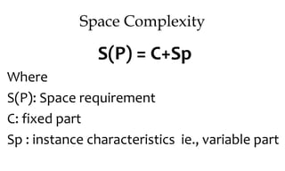
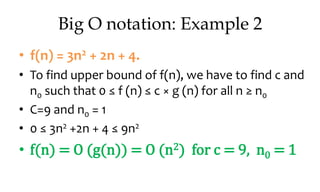
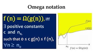
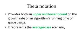
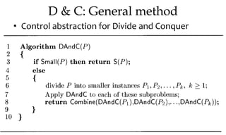
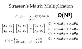
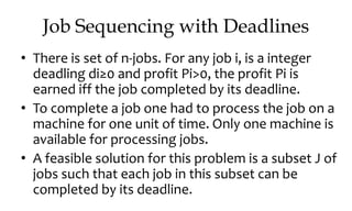
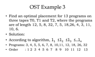
![Greedy algorithm for knapsack
Algorithm GreedyKnapsack(m,n)
// p[i:n] and [1:n] contain the profits and weights respectively
// if the n-objects ordered such that p[i]/w[i]>=p[i+1]/w[i+1],
m size of knapsack and x[1:n] the solution vector
{
for i:=1 to n do x[i]:=0.0
U:=m;
for i:=1 to n do
{
if(w[i]>U) then break;
x[i]:=1.0;
U:=U-w[i];
}
if(i<=n) then x[i]:=U/w[i];
}](https://image.slidesharecdn.com/daapost-240405134921-2dcf40bc/85/Design-and-Analysis-of-Algorithms-Lecture-Notes-75-320.jpg)
![Algorithm GreedyKnapsack(m,n)
{
for i:=1 to n do x[i]:=0.0
U:=m;
for i:=1 to n do
{
if(w[i]>U) then break;
x[i]:=1.0;
U:=U-w[i];
}
if(i<=n) then x[i]:=U/w[i];
}
X[1]=x[2]=x[3]=x[4]=x[5]=x[6]=0
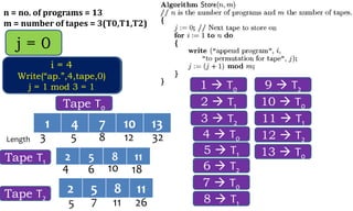
n=6, p=(18, 5, 9, 10, 12, 7), w=(7, 2, 3, 5, 3, 2), M=13
U=13
i=1
3>13 false
X[1]=1
U=13-3=10
i=2
2>10 false
X[2]=1
U=10-2=8
i=3
3>8 false
X[3]=1
U=8-3=5
i=4
7>5 True
break
X[4]= 5 ÷ 7
Profit = Profit (X1+X2+X3+(5/7)*X4) = 12+7+9+12.85 = 40.85](https://image.slidesharecdn.com/daapost-240405134921-2dcf40bc/85/Design-and-Analysis-of-Algorithms-Lecture-Notes-76-320.jpg)
![JSD: Algorithm
• The value of a feasible solution J is the sum of the profits of
the jobs in J, i.e., ∑i∈jPi
• An optimal solution is a feasible solution with maximum
value.
//d dead line, jsubset of jobs ,n total
number of jobs
// d[i]≥1, 1 ≤ i ≤ n are the dead lines,
// the jobs are ordered such that p[1]≥p[2]≥---
≥p[n]
• //j[i] is the ith job in the optimal solution
1 ≤ i ≤ k, k subset range](https://image.slidesharecdn.com/daapost-240405134921-2dcf40bc/85/Design-and-Analysis-of-Algorithms-Lecture-Notes-79-320.jpg)
![algorithm js(d, j, n)
{
d[0]=j[0]=0;j[1]=1;k=1;
for i=2 to n do {
r=k;
while((d[j[r]]>d[i]) and [d[j[r]]≠r)) do
r=r-1;
if((d[j[r]]≤d[i]) and (d[i]> r)) then
{
for q:=k to (r+1) step-1 do j[q+1]= j[q];
j[r+1]=i;
k=k+1;
}
}
Job Sequencing with
Deadlines: Algorithm](https://image.slidesharecdn.com/daapost-240405134921-2dcf40bc/85/Design-and-Analysis-of-Algorithms-Lecture-Notes-80-320.jpg)
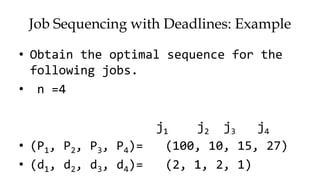
![Let n =5; P = { 20, 15, 10, 5, 1 } and D = { 2, 2, 1, 3, 3 }
d[0] = 0; j[0]= 0;
j[1] = 1; k = 1
i=2
r=k=1
while(2>2 False
if(2<=2 and (2>1) True
{
for(q=k;q>=r+1;q--) False
j[2] = 2
k = 2
i=3
r=k=2
while( False
if(2<=1 and (1>2) False
i=4
r=k=2
while( False
if(2<=3 and (3>2) True
for(q=k;q>=r+1;q--) False
j[3] = 4
k=3
i=5
r=k=3
while( False
i=6 to 5 False
Sequence of Jobs : (J1, J2, J4)
Profit : p1+p2+p4 = 40
if(1<=3 and (3>3) False](https://image.slidesharecdn.com/daapost-240405134921-2dcf40bc/85/Design-and-Analysis-of-Algorithms-Lecture-Notes-81-320.jpg)
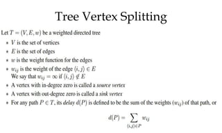
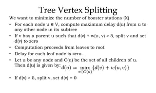
![Tree Vertex Splitting
• Delay of tree T , d(T ) is maximum of all path delays
• Splitting vertices to create forest
• ∗ Let T /X be the forest that results when each vertex
u ∈ X is split into two nodes ui and uo such that all
the edges 〈u, j〉 ∈ E [〈j, u〉 ∈ E] are replaced by
edges of the form 〈uo, j〉 ∈ E [〈j, ui〉 ∈ E]
• Outbound edges from u now leave from uo
• Inbound edges to u now enter at ui
• ∗ Split node is the booster station](https://image.slidesharecdn.com/daapost-240405134921-2dcf40bc/85/Design-and-Analysis-of-Algorithms-Lecture-Notes-84-320.jpg)
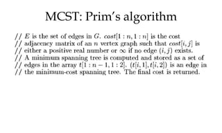
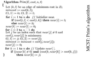
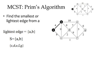
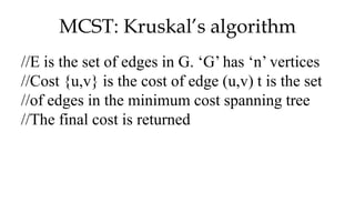
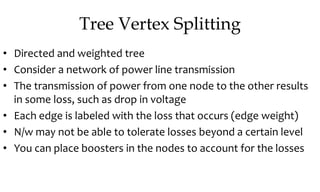
![MCST: Kruskals algorithm
Algorithm Kruskal (E, cost, n,t)
{
construct a heap out of the edge costs using heapify;
for i:= 1 to n do parent (i):= -1
i: = 0; min cost: = 0.0;
While (i<n-1) and (heap not empty)) do
{
Delete a minimum cost edge (u,v) from the heaps; and reheapify using adjust;
j:= find (u); k:=find (v);
if (jk) then
{ i: = 1+1; t [i,1] = u; t [i,2] =v; mincost: =mincost+cost(u,v); Union (j,k); }
}
if (in-1) then write (“No spanning tree”); else return mincost;
}](https://image.slidesharecdn.com/daapost-240405134921-2dcf40bc/85/Design-and-Analysis-of-Algorithms-Lecture-Notes-103-320.jpg)
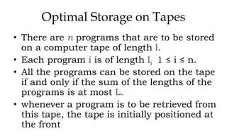
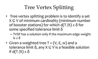
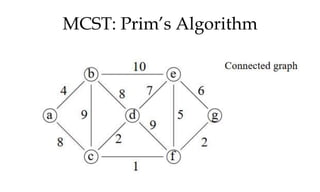
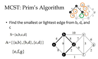
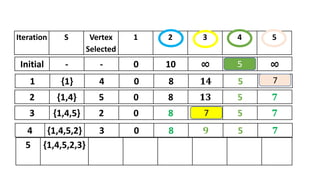
![2
1
3
4 5
i = 1 to 5
S[1] = false; dist[1]=cost[1,1] dist[1]=0
S[2] = false; dist[2]=cost[1,2] dist[2]=10
S[3] = false; dist[3]=cost[1,3] dist[3]=∞
S[4] = false; dist[4]=cost[1,4] dist[4]=5
S[5] = false; dist[5]=cost[1,5] dist[5]= ∞
S[1] = true; dist[1] = 0
dist[ 1] 0 0 0 0
dist[ 2] 10 8 8 8
dist[ 3] ∞ 14 13 9
dist[ 4] 5 5 5 5
dist[ 5] ∞ 7 7 7
S
{1}
{1,4}
{1,4,5}
{1,4,5,2}
{1,4,5,2,3}
dist[ 1] 0
dist[ 2] 8
dist[ 3] 9
dist[ 4] 5
dist[ 5] 7](https://image.slidesharecdn.com/daapost-240405134921-2dcf40bc/85/Design-and-Analysis-of-Algorithms-Lecture-Notes-120-320.jpg)

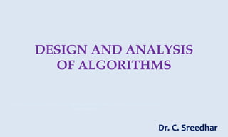
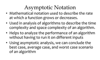
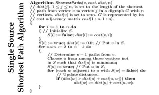
This document discusses algorithms and their analysis. It begins by defining an algorithm and its key characteristics like being finite, definite, and terminating after a finite number of steps. It then discusses designing algorithms to minimize cost and analyzing algorithms to predict their performance. Various algorithm design techniques are covered like divide and conquer, binary search, and its recursive implementation. Asymptotic notations like Big-O, Omega, and Theta are introduced to analyze time and space complexity. Specific algorithms like merge sort, quicksort, and their recursive implementations are explained in detail.