Downloaded 51 times

![Input Parameters:
Cross validation
# Specify 5-fold cross validation
model_with_5folds = h2o.glm(data = h2odf, y = y, x = x, family = "binomial",
nfolds = 5)
print(model_with_5folds@model$auc)
print(model_with_5folds@xval[[1]]@model$auc)
print(model_with_5folds@xval[[2]]@model$auc)
print(model_with_5folds@xval[[3]]@model$auc)
print(model_with_5folds@xval[[4]]@model$auc)
print(model_with_5folds@xval[[5]]@model$auc)
H2O.ai
Machine Intelligence](https://image.slidesharecdn.com/distributedglmtk20150127atl-150130130722-conversion-gate01/85/Distributed-GLM-with-H2O-Atlanta-Meetup-22-320.jpg)
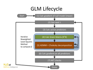
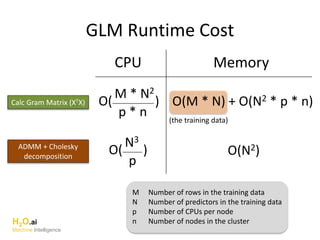
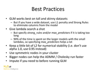
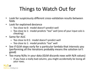
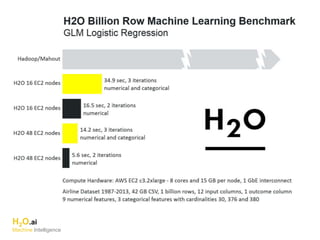

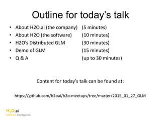
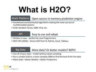
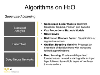
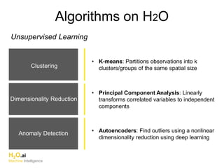
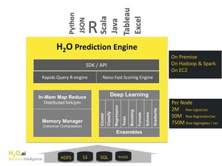
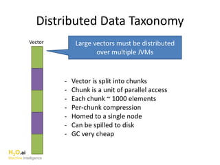
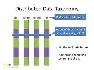
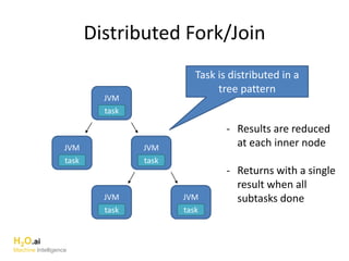
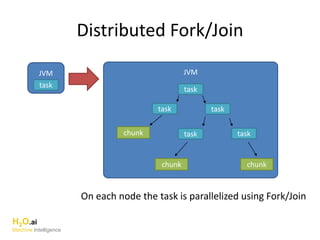
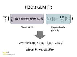
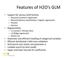
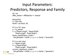
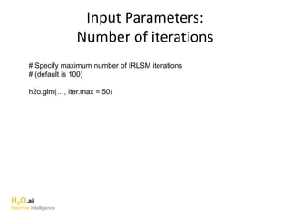
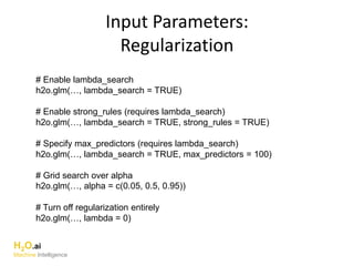
The document outlines a presentation about H2O's distributed generalized linear model (GLM) algorithm. The presentation includes sections about H2O.ai the company, an overview of the H2O software, a 30 minute section explaining H2O's distributed GLM in detail, a 15 minute demo of GLM, and a question and answer period. The document provides background on H2O.ai and H2O, and outlines the topics that will be covered in the distributed GLM section, including the algorithm, input parameters, outputs, runtime costs, and best practices.


![20260201 [FOSDEM] gomodjail - library sandboxing for Go modules.pdf](https://cdn.slidesharecdn.com/ss_thumbnails/20260201fosdemgomodjail-librarysandboxingforgomodules-260201225659-76609ec4-thumbnail.jpg?width=640&height=640&fit=bounds)


