Download as PDF, PPTX


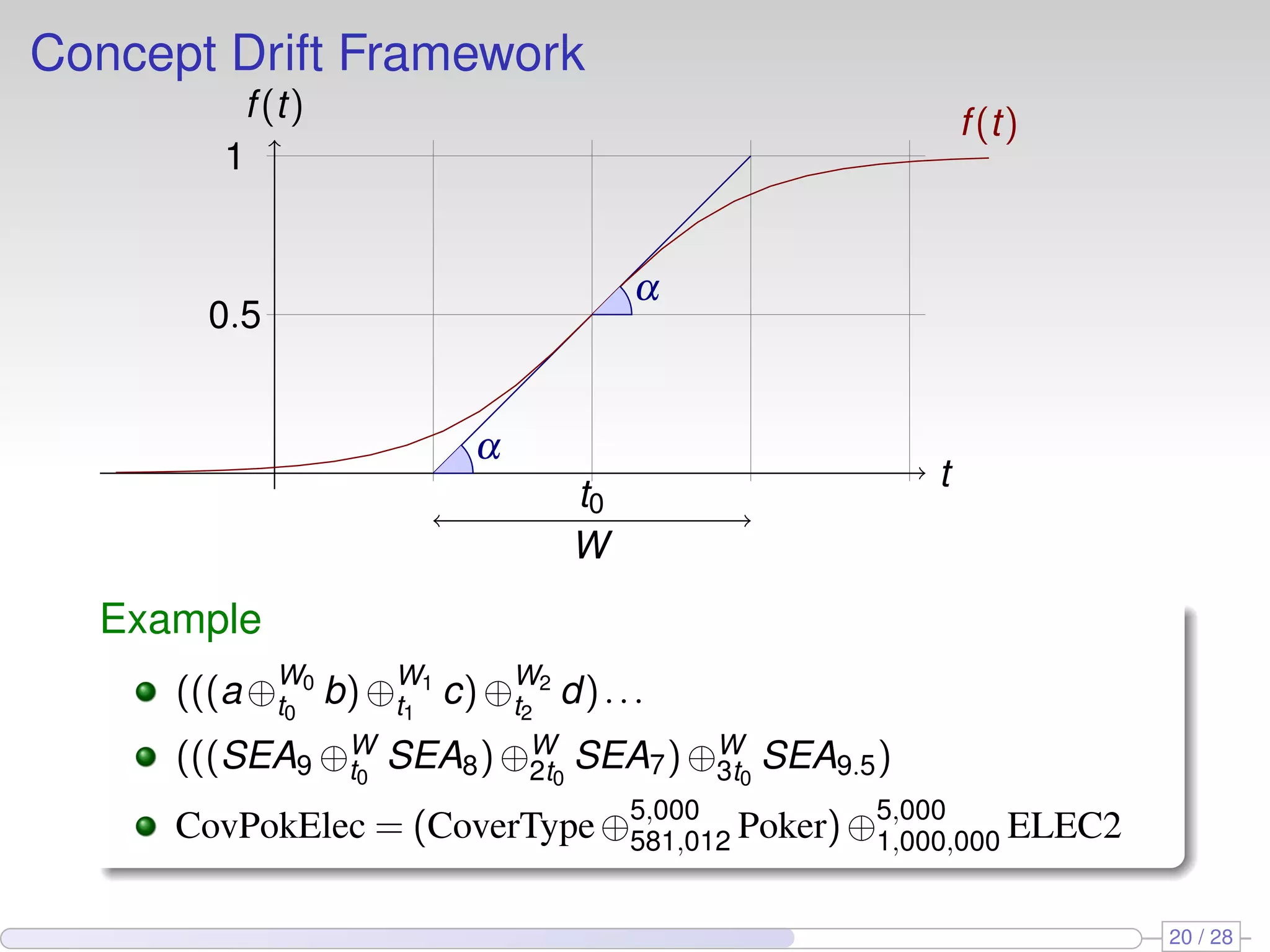
![Concept Drift Framework
t
f(t) f(t)
α
α
t0
W
0.5
1
Definition
Given two data streams a, b, we define c = a⊕W
t0
b as the data
stream built joining the two data streams a and b
Pr[c(t) = b(t)] = 1/(1+e−4(t−t0)/W ).
Pr[c(t) = a(t)] = 1−Pr[c(t) = b(t)]
20 / 28](https://image.slidesharecdn.com/pakdd10-101101164426-phpapp01/75/Fast-Perceptron-Decision-Tree-Learning-from-Evolving-Data-Streams-25-2048.jpg)
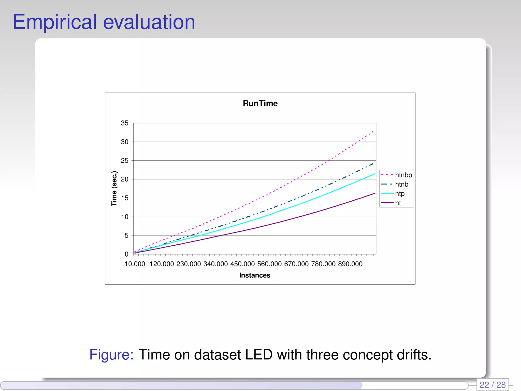
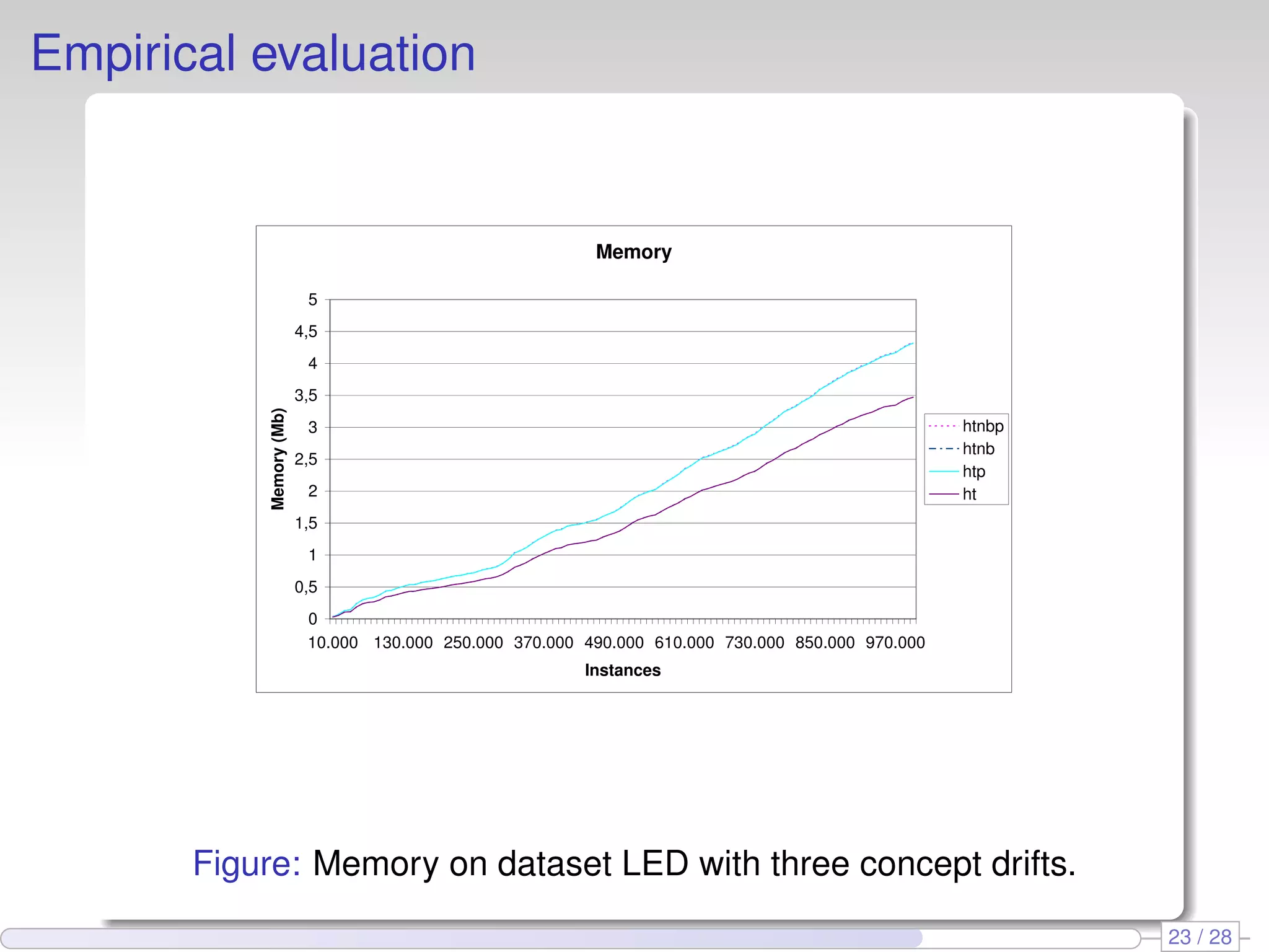
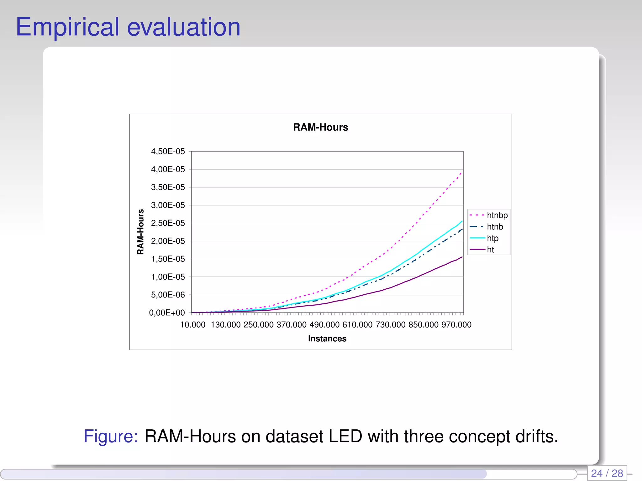
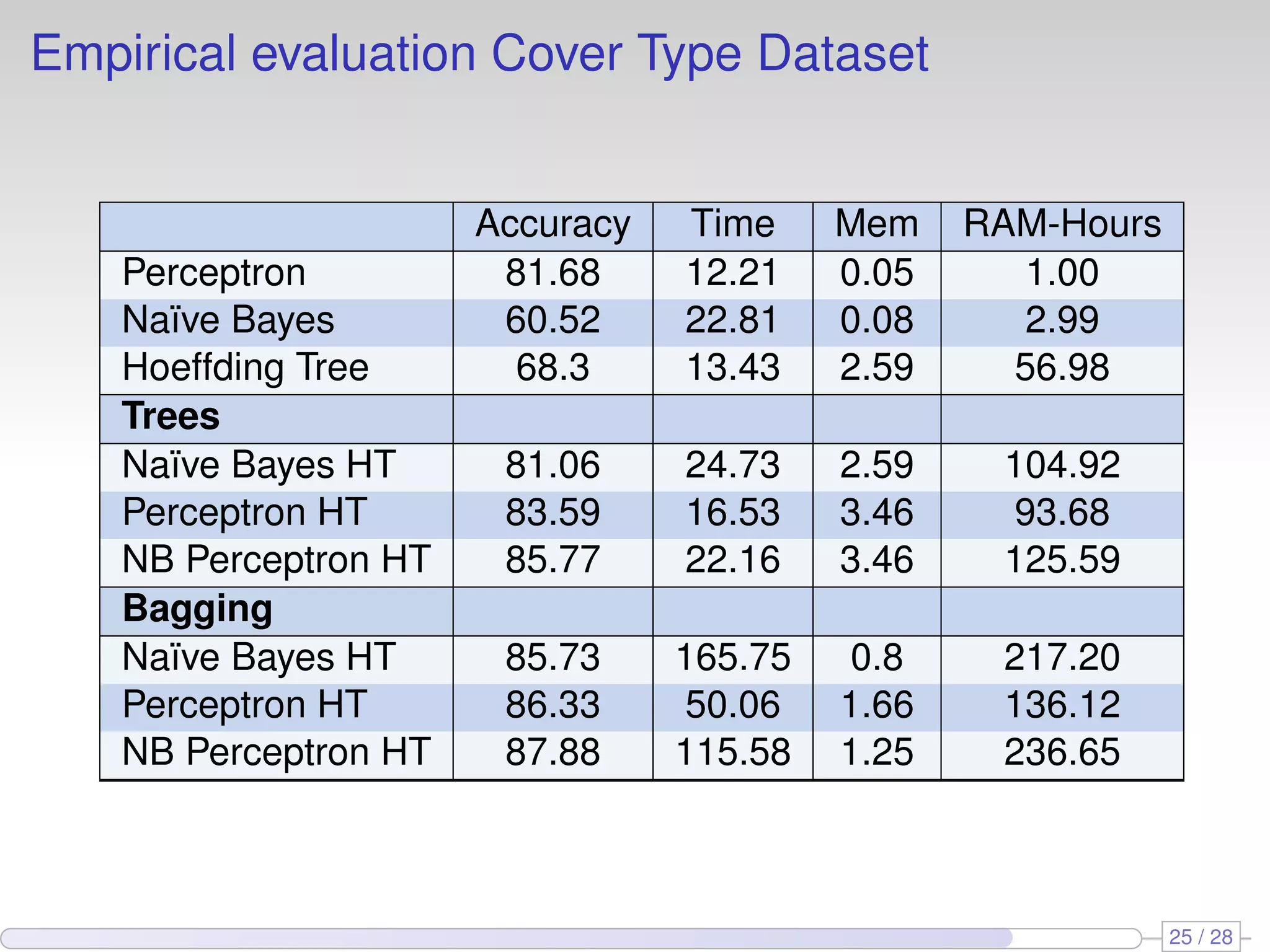
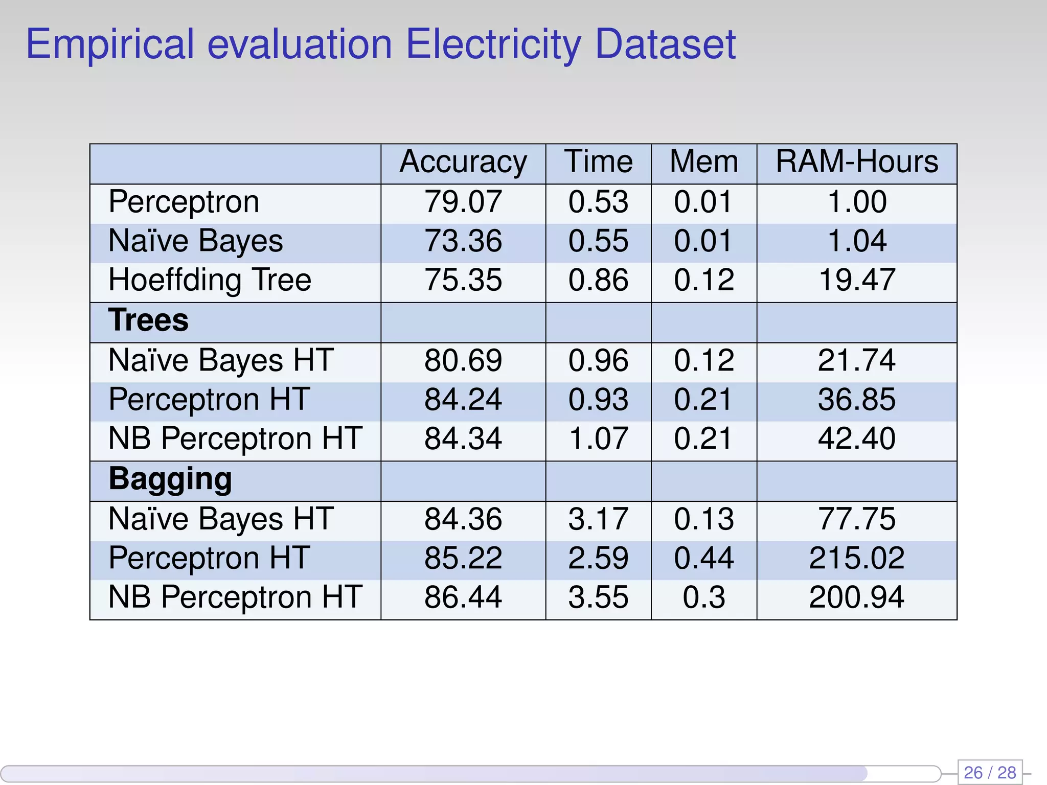

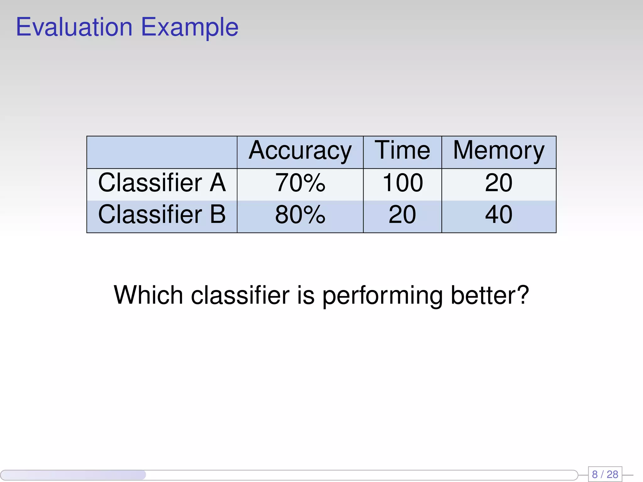
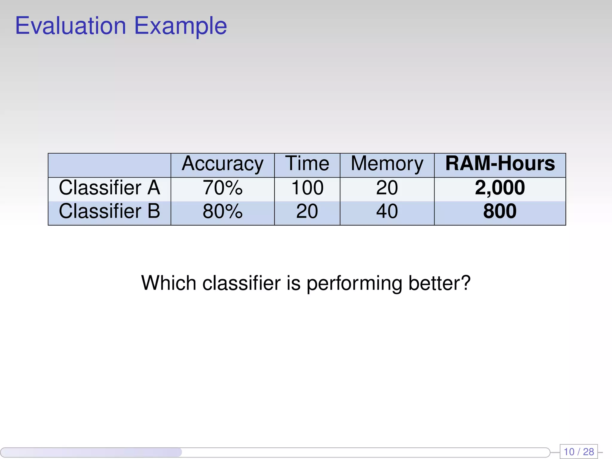
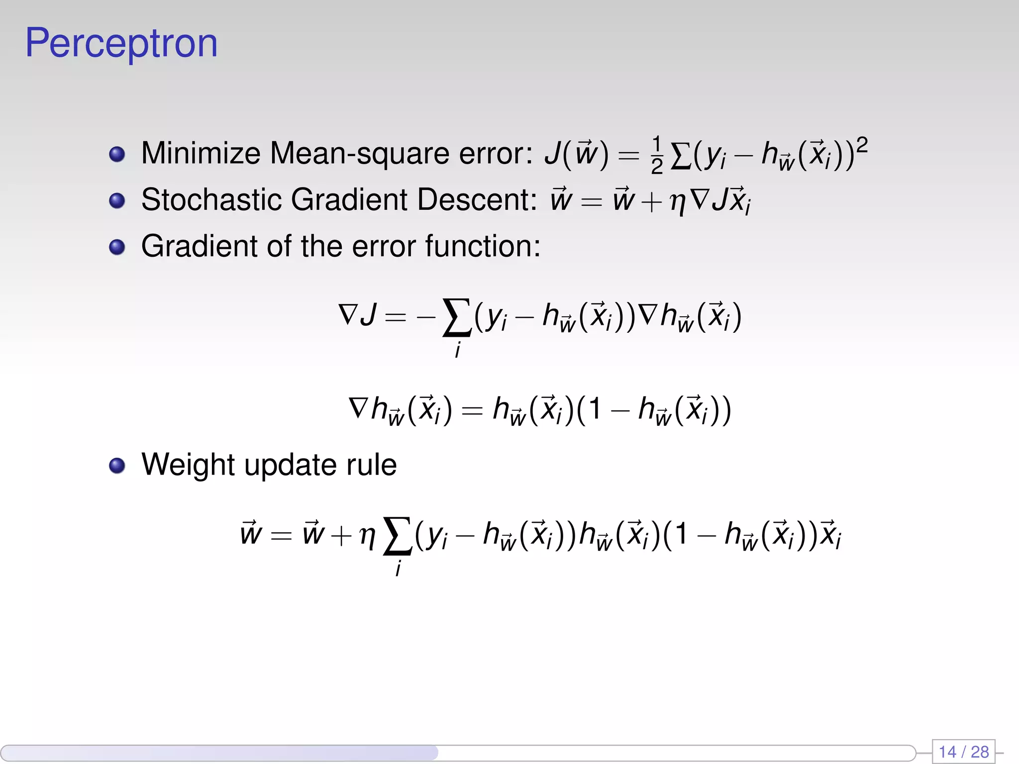
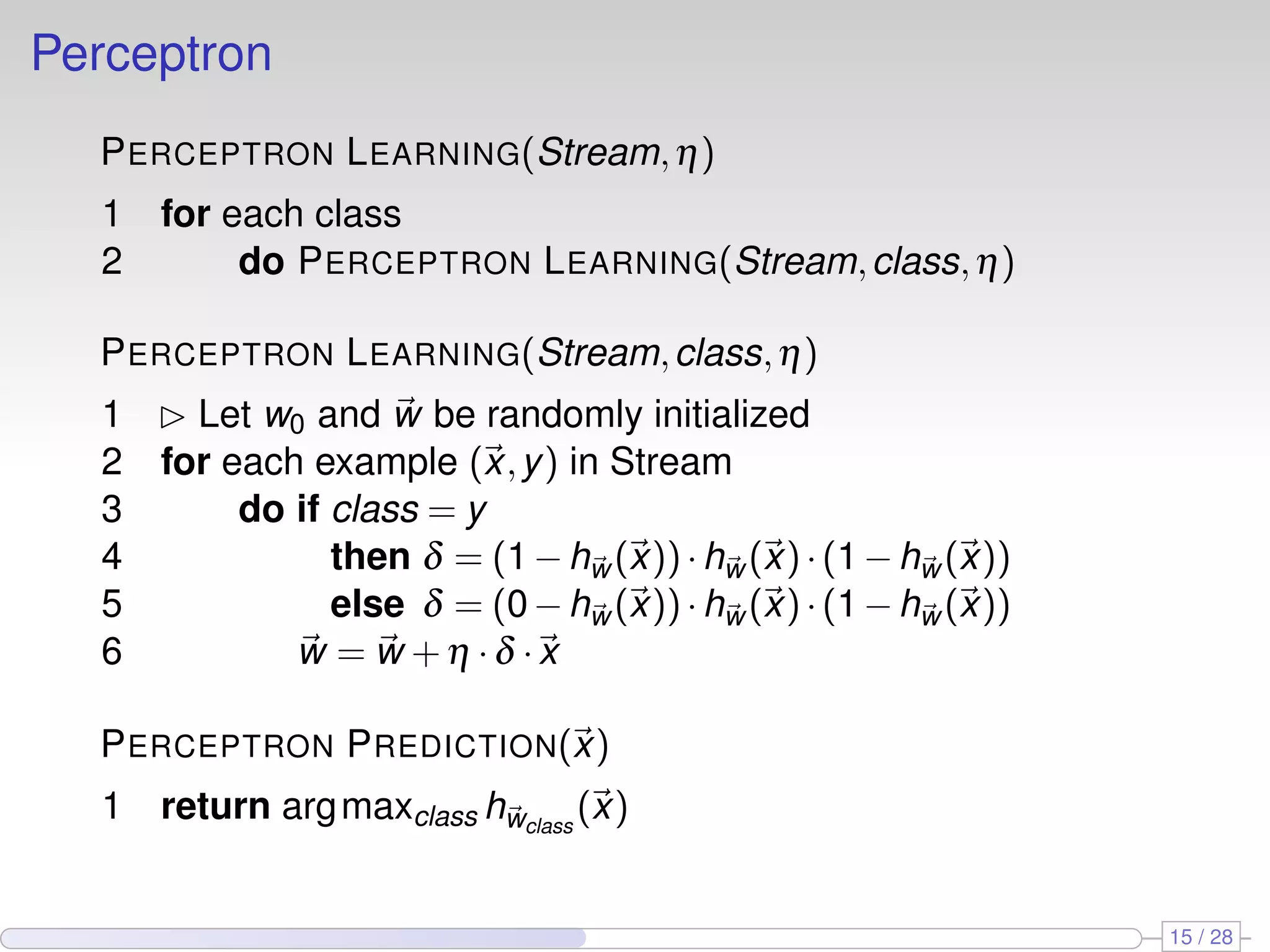
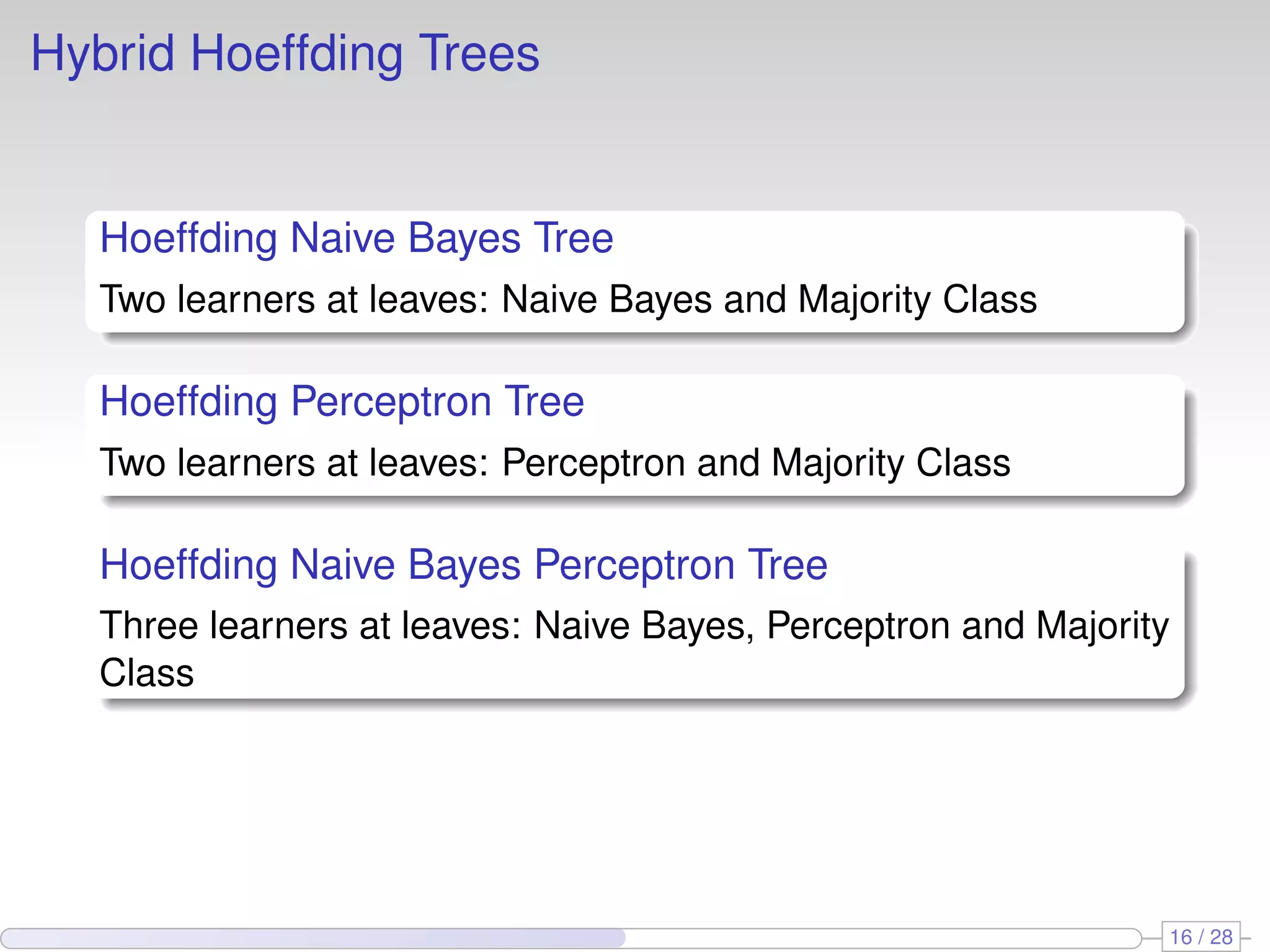
The document proposes using perceptron learners at the leaves of Hoeffding decision trees to improve performance on data streams. It introduces a new evaluation metric called RAM-Hours that considers both time and memory usage. The authors empirically evaluate different classifier models, including Hoeffding trees with perceptron and naive Bayes learners at leaves, on several datasets. Results show that hybrid models like Hoeffding naive Bayes perceptron trees often provide the best balance of accuracy, time and memory usage.


![[ppt]](https://cdn.slidesharecdn.com/ss_thumbnails/ppt2931-thumbnail.jpg?width=640&height=640&fit=bounds)
![[ppt]](https://cdn.slidesharecdn.com/ss_thumbnails/ppt3441-thumbnail.jpg?width=640&height=640&fit=bounds)


![Vibe Coding vs. Spec-Driven Development [Free Meetup]](https://cdn.slidesharecdn.com/ss_thumbnails/vibecodingvsspecdrivendevelopment-251209105622-43f455e7-thumbnail.jpg?width=640&height=640&fit=bounds)


