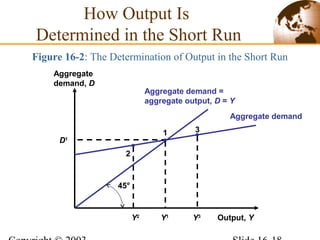
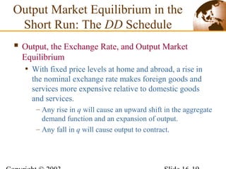
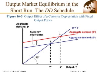
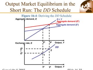
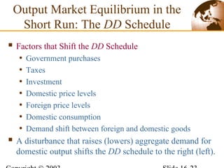
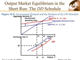
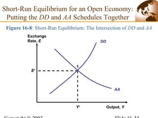
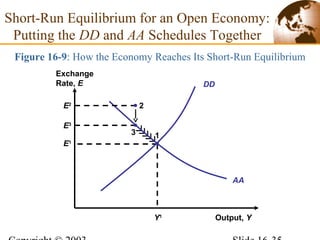
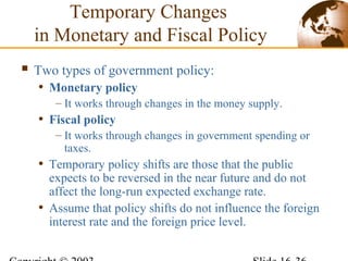
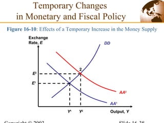
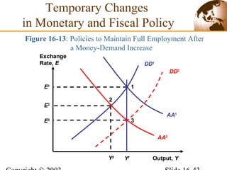
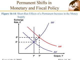
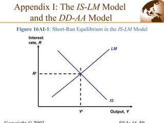
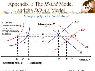
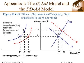
This chapter discusses output and exchange rates in the short run for an open economy. It introduces models of aggregate demand and asset market equilibrium. The DD schedule shows combinations of output and exchange rates where the output market is in equilibrium. The AA schedule shows combinations where the money and foreign exchange markets are in equilibrium. Short-run macroeconomic equilibrium occurs at the intersection of the DD and AA schedules. The effects of temporary and permanent monetary and fiscal policy shifts are analyzed using the model. Policy tools can be used to maintain full employment in response to short-run disturbances.
Determination of exchange rate chapter 6Nayan Vaghela
Determination of exchange rate, mint par theory, balance of payment theory, Purchasing power parity theory, Absolute version and relative version, Criticisms
Indian Currency Exchange rate of foreign currency relating to imported and ex...Jhunjhunwalas
In exercise of the powers conferred by Section 14 of the Customs Act, 1962 (52 of 1962), and in super session of the notification of the Government of India in the Ministry of Finance (Department of Revenue) No.47/2014-CUSTOMS (N.T.), dated the 19th June, 2014 vide number S.O.1565(E), dated the 19th June, 2014, except as respects things done or omitted to be done before such supersession, the Central Board of Excise and Customs (CBEC) hereby determines that the rate of exchange of conversion of each of the foreign currency specified in column (2) of each of Schedule I and Schedule II annexed hereto into Indian currency or vice versa shall be with effect from 4th July, 2014 be the rate mentioned against it in the corresponding entry in column (3) thereof, for the purpose of the said section, relating to imported and export goods.
it describes the bony anatomy including the femoral head , acetabulum, labrum . also discusses the capsule , ligaments . muscle that act on the hip joint and the range of motion are outlined. factors affecting hip joint stability and weight transmission through the joint are summarized.
Delivering Micro-Credentials in Technical and Vocational Education and TrainingAG2 Design
Explore how micro-credentials are transforming Technical and Vocational Education and Training (TVET) with this comprehensive slide deck. Discover what micro-credentials are, their importance in TVET, the advantages they offer, and the insights from industry experts. Additionally, learn about the top software applications available for creating and managing micro-credentials. This presentation also includes valuable resources and a discussion on the future of these specialised certifications.
For more detailed information on delivering micro-credentials in TVET, visit this https://tvettrainer.com/delivering-micro-credentials-in-tvet/
How to Add Chatter in the odoo 17 ERP ModuleCeline George
In Odoo, the chatter is like a chat tool that helps you work together on records. You can leave notes and track things, making it easier to talk with your team and partners. Inside chatter, all communication history, activity, and changes will be displayed.
This presentation includes basic of PCOS their pathology and treatment and also Ayurveda correlation of PCOS and Ayurvedic line of treatment mentioned in classics.
A workshop hosted by the South African Journal of Science aimed at postgraduate students and early career researchers with little or no experience in writing and publishing journal articles.
June 3, 2024 Anti-Semitism Letter Sent to MIT President Kornbluth and MIT Cor...Levi Shapiro
Letter from the Congress of the United States regarding Anti-Semitism sent June 3rd to MIT President Sally Kornbluth, MIT Corp Chair, Mark Gorenberg
Dear Dr. Kornbluth and Mr. Gorenberg,
The US House of Representatives is deeply concerned by ongoing and pervasive acts of antisemitic
harassment and intimidation at the Massachusetts Institute of Technology (MIT). Failing to act decisively to ensure a safe learning environment for all students would be a grave dereliction of your responsibilities as President of MIT and Chair of the MIT Corporation.
This Congress will not stand idly by and allow an environment hostile to Jewish students to persist. The House believes that your institution is in violation of Title VI of the Civil Rights Act, and the inability or
unwillingness to rectify this violation through action requires accountability.
Postsecondary education is a unique opportunity for students to learn and have their ideas and beliefs challenged. However, universities receiving hundreds of millions of federal funds annually have denied
students that opportunity and have been hijacked to become venues for the promotion of terrorism, antisemitic harassment and intimidation, unlawful encampments, and in some cases, assaults and riots.
The House of Representatives will not countenance the use of federal funds to indoctrinate students into hateful, antisemitic, anti-American supporters of terrorism. Investigations into campus antisemitism by the Committee on Education and the Workforce and the Committee on Ways and Means have been expanded into a Congress-wide probe across all relevant jurisdictions to address this national crisis. The undersigned Committees will conduct oversight into the use of federal funds at MIT and its learning environment under authorities granted to each Committee.
• The Committee on Education and the Workforce has been investigating your institution since December 7, 2023. The Committee has broad jurisdiction over postsecondary education, including its compliance with Title VI of the Civil Rights Act, campus safety concerns over disruptions to the learning environment, and the awarding of federal student aid under the Higher Education Act.
• The Committee on Oversight and Accountability is investigating the sources of funding and other support flowing to groups espousing pro-Hamas propaganda and engaged in antisemitic harassment and intimidation of students. The Committee on Oversight and Accountability is the principal oversight committee of the US House of Representatives and has broad authority to investigate “any matter” at “any time” under House Rule X.
• The Committee on Ways and Means has been investigating several universities since November 15, 2023, when the Committee held a hearing entitled From Ivory Towers to Dark Corners: Investigating the Nexus Between Antisemitism, Tax-Exempt Universities, and Terror Financing. The Committee followed the hearing with letters to those institutions on January 10, 202
A Strategic Approach: GenAI in EducationPeter Windle
Artificial Intelligence (AI) technologies such as Generative AI, Image Generators and Large Language Models have had a dramatic impact on teaching, learning and assessment over the past 18 months. The most immediate threat AI posed was to Academic Integrity with Higher Education Institutes (HEIs) focusing their efforts on combating the use of GenAI in assessment. Guidelines were developed for staff and students, policies put in place too. Innovative educators have forged paths in the use of Generative AI for teaching, learning and assessments leading to pockets of transformation springing up across HEIs, often with little or no top-down guidance, support or direction.
This Gasta posits a strategic approach to integrating AI into HEIs to prepare staff, students and the curriculum for an evolving world and workplace. We will highlight the advantages of working with these technologies beyond the realm of teaching, learning and assessment by considering prompt engineering skills, industry impact, curriculum changes, and the need for staff upskilling. In contrast, not engaging strategically with Generative AI poses risks, including falling behind peers, missed opportunities and failing to ensure our graduates remain employable. The rapid evolution of AI technologies necessitates a proactive and strategic approach if we are to remain relevant.
Macroeconomics- Movie Location
This will be used as part of your Personal Professional Portfolio once graded.
Objective:
Prepare a presentation or a paper using research, basic comparative analysis, data organization and application of economic information. You will make an informed assessment of an economic climate outside of the United States to accomplish an entertainment industry objective.
Read| The latest issue of The Challenger is here! We are thrilled to announce that our school paper has qualified for the NATIONAL SCHOOLS PRESS CONFERENCE (NSPC) 2024. Thank you for your unwavering support and trust. Dive into the stories that made us stand out!
Biological screening of herbal drugs: Introduction and Need for
Phyto-Pharmacological Screening, New Strategies for evaluating
Natural Products, In vitro evaluation techniques for Antioxidants, Antimicrobial and Anticancer drugs. In vivo evaluation techniques
for Anti-inflammatory, Antiulcer, Anticancer, Wound healing, Antidiabetic, Hepatoprotective, Cardio protective, Diuretics and
Antifertility, Toxicity studies as per OECD guidelines
1. Chapter 16Chapter 16
Output and the Exchange Rate in the Short RunOutput and the Exchange Rate in the Short Run
Prepared by Iordanis Petsas
To Accompany
International Economics: Theory and PolicyInternational Economics: Theory and Policy, Sixth Edition
by Paul R. Krugman and Maurice Obstfeld
2. Chapter Organization
Determinants of Aggregate Demand in an Open
Economy
The Equation of Aggregate Demand
How Output Is Determined in the Short Run
Output Market Equilibrium in the Sort Run: The DD
Schedule
Asset Market Equilibrium in the Short Run: The AA
Schedule
Short-Run Equilibrium for an Open Economy:
Putting the DD and AA Schedules Together
3. Temporary Changes in Monetary and Fiscal Policy
Inflation Bias and Other Problems of Policy
Formulation
Permanent Shifts in Monetary and Fiscal Policy
Macroeconomic Policies and the Current Account
Gradual Trade Flow Adjustment and Current Account
Dynamics
Summary
Chapter Organization
4. Appendix I: The IS-LM Model and the DD-AA Model
Appendix II: Intertemporal Trade and Consumption
Demand
Appendix III: The Marshall-Lerner Condition and
Empirical Estimates of Trade Elasticities
Chapter Organization
5. Introduction
Macroeconomic changes that affect exchange rates,
interest rates, and price levels may also affect output.
• This chapter introduces a new theory of how the
output market adjusts to demand changes when
product prices are themselves slow to adjust.
A short-run model of the output market in an open
economy will be utilized to analyze:
• The effects of macroeconomic policy tools on output
and the current account
• The use of macroeconomic policy tools to maintain
full employment
6. Determinants of Aggregate
Demand in an Open Economy
Aggregate demand
• The amount of a country’s goods and services
demanded by households and firms throughout the
world.
The aggregate demand for an open economy’s output
consists of four components:
• Consumption demand (C)
• Investment demand (I)
• Government demand (G)
• Current account (CA)
7. Determinants of Consumption Demand
• Consumption demand increases as disposable income
(i.e., national income less taxes) increases at the
aggregate level.
– The increase in consumption demand is less than the
increase in the disposable income because part of the
income increase is saved.
Determinants of Aggregate
Demand in an Open Economy
8. Determinants of the Current Account
• The CA balance is viewed as the demand for a
country’s exports (EX) less that country's own demand
for imports (IM).
• The CA balance is determined by two main factors:
– The domestic currency’s real exchange rate against
foreign currency (q = EP*/P)
– Domestic disposable income (Yd
)
Determinants of Aggregate
Demand in an Open Economy
9. How Real Exchange Rate Changes Affect the Current
Account
• An increase in q raises EX and improves the domestic
country’s CA.
– Each unit of domestic output now purchases fewer units
of foreign output, therefore, foreign will demand more
exports.
• An increase q can raise or lower IM and has an
ambiguous effect on CA.
– IM denotes the value of imports measured in terms of
domestic output.
Determinants of Aggregate
Demand in an Open Economy
10. There are two effects of a real exchange rate:
• Volume effect
– The effect of consumer spending shifts on export and
import quantities
• Value effect
– It changes the domestic output worth of a given volume
of foreign imports.
Whether the CA improves or worsens depends on
which effect of a real exchange rate change is
dominant.
We assume that the volume effect of a real exchange
rate change always outweighs the value effect.
Determinants of Aggregate
Demand in an Open Economy
11. How Disposable Income Changes Affect the Current
Account
• An increase in disposable income (Yd
) worsens the CA.
• A rise in Yd
causes domestic consumers to increase their
spending on all goods.
Determinants of Aggregate
Demand in an Open Economy
13. The four components of aggregate demand are
combined to get the total aggregate demand:
D = C(Y – T) + I + G + CA(EP*/P, Y – T)
This equation shows that aggregate demand for home
output can be written as:
D = D(EP*/P, Y – T, I, G)
The Equation of Aggregate Demand
14. The Real Exchange Rate and Aggregate Demand
• An increase in q raises CA and D.
– It makes domestic goods and services cheaper relative
to foreign goods and services.
– It shifts both domestic and foreign spending from
foreign goods to domestic goods.
– A real depreciation of the home currency raises
aggregate demand for home output.
– A real appreciation lowers aggregate demand for home output.
The Equation of Aggregate Demand
15. Real Income and Aggregate Demand
• A rise in domestic real income raises aggregate
demand for home output.
• A fall in domestic real income lowers aggregate
demand for home output.
The Equation of Aggregate Demand
16. Figure 16-1: Aggregate Demand as a Function of Output
Output (real income), Y
Aggregate
demand, D
Aggregate demand function,
D(EP*/P, Y – T, I, G)
45°
The Equation of Aggregate Demand
17. How Output Is
Determined in the Short Run
Output market is in equilibrium in the short-run when
real output, Y, equals the aggregate demand for
domestic output:
Y = D(EP*/P, Y – T, I, G) (16-1)
18. Figure 16-2: The Determination of Output in the Short Run
Output, Y
Aggregate
demand, D
45°
Aggregate demand =
aggregate output, D = Y
Aggregate demand
2
Y2
D1
1
Y1
3
Y3
How Output Is
Determined in the Short Run
19. Output, the Exchange Rate, and Output Market
Equilibrium
• With fixed price levels at home and abroad, a rise in
the nominal exchange rate makes foreign goods and
services more expensive relative to domestic goods
and services.
– Any rise in q will cause an upward shift in the aggregate
demand function and an expansion of output.
– Any fall in q will cause output to contract.
Output Market Equilibrium in the
Short Run: The DD Schedule
20. Output Market Equilibrium in the
Short Run: The DD Schedule
Figure 16-3: Output Effect of a Currency Depreciation with Fixed
Output Prices
Output, Y
Aggregate
demand, D
45°
D = Y
1
Y1
Aggregate demand (E2
)
Aggregate demand (E1
)
Y2
2
Currency
depreciates
21. Deriving the DD Schedule
• DD schedule
– It shows all combinations of output and the exchange
rate for which the output market is in short-run
equilibrium (aggregate demand = aggregate output).
– It slopes upward because a rise in the exchange rate
causes output to rise.
Output Market Equilibrium in the
Short Run: The DD Schedule
22. Y2
DD
Output Market Equilibrium in the
Short Run: The DD Schedule
Figure 16-4: Deriving the DD Schedule
Output, Y
Aggregate demand, D D = Y
Y1
Aggregate demand (E2
)
Aggregate demand (E1
)
Y2
Output, Y
Exchange rate, E
Y1
1
E1
E2
2
23. Factors that Shift the DD Schedule
• Government purchases
• Taxes
• Investment
• Domestic price levels
• Foreign price levels
• Domestic consumption
• Demand shift between foreign and domestic goods
A disturbance that raises (lowers) aggregate demand for
domestic output shifts the DD schedule to the right (left).
Output Market Equilibrium in the
Short Run: The DD Schedule
24. Y2
Output Market Equilibrium in the
Short Run: The DD Schedule
Figure 16-5: Government Demand and the Position of the DD Schedule
D = Y
Y1
D(E0
P*/P, Y – T, I, G2
)
D(E0
P*/P, Y – T, I, G1
)
Y2
Output, Y
Exchange rate, E
Y1
Aggregate demand curves
2
Government
spending rises
Output, Y
Aggregate demand, D
DD1
E0
1
DD2
25. AA Schedule
• It shows all combinations of exchange rate and output
that are consistent with equilibrium in the domestic
money market and the foreign exchange market.
Asset Market Equilibrium in the
Short Run: The AA Schedule
26. Output, the Exchange Rate, and Asset Market
Equilibrium
• We will combine the interest parity condition with the
money market to derive the asset market equilibrium
in the short-run.
• The interest parity condition describing foreign
exchange market equilibrium is:
R = R* + (Ee
– E)/E
where: Ee
is the expected future exchange rate
R is the interest rate on domestic currency deposits
R*
is the interest rate on foreign currency deposits
Asset Market Equilibrium in the
Short Run: The AA Schedule
27. • The R satisfying the interest parity condition must also
equate the real domestic money supply to aggregate
real money demand:
Ms
/P = L(R, Y)
• Aggregate real money demand L(R, Y) rises when the
interest rate falls because a fall in R makes interest-
bearing nonmoney assets less attractive to hold.
Asset Market Equilibrium in the
Short Run: The AA Schedule
28. Asset Market Equilibrium in the
Short Run: The AA ScheduleFigure 16-6: Output and the Exchange Rate in Asset Market
Equilibrium
Domestic-currency
return on foreign-
currency deposits
Foreign
exchange
market
Money
market
E2
2'
R2
E1
1'
R1
Real money
supply
MS
P
1
L(R, Y2
)
L(R, Y1
)
Real domestic money holdings
Domestic
interest
rate, R
Exchange Rate, E
0
2
Output rises
29. For asset markets to remain in equilibrium:
• A rise in domestic output must be accompanied by an
appreciation of the domestic currency.
• A fall in domestic output must be accompanied by a
depreciation of the domestic currency.
Asset Market Equilibrium in the
Short Run: The AA Schedule
30. Deriving the AA Schedule
• It relates exchange rates and output levels that keep the
money and foreign exchange markets in equilibrium.
• It slopes downward because a rise in output causes a
rise in the home interest rate and a domestic currency
appreciation.
Asset Market Equilibrium in the
Short Run: The AA Schedule
31. Figure 16-7: The AA Schedule
Output, Y
Exchange
Rate, E
Asset Market Equilibrium in the
Short Run: The AA Schedule
AA
Y1
E1
1
Y2
E2
2
32. Factors that Shift the AA Schedule
• Domestic money supply
• Domestic price level
• Expected future exchange rate
• Foreign interest rate
• Shifts in the aggregate real money demand schedule
Asset Market Equilibrium in the
Short Run: The AA Schedule
33. Short-Run Equilibrium for an Open Economy:
Putting the DD and AA Schedules Together
A short-run equilibrium for the economy as a whole
must bring equilibrium simultaneously in the output
and asset markets.
• That is, it must lie on both DD and AA schedules.
34. Figure 16-8: Short-Run Equilibrium: The Intersection of DD and AA
Output, Y
Exchange
Rate, E
AA
Y1
E1
1
Short-Run Equilibrium for an Open Economy:
Putting the DD and AA Schedules Together
DD
35. Figure 16-9: How the Economy Reaches Its Short-Run Equilibrium
AA
Y1
E1
1
Short-Run Equilibrium for an Open Economy:
Putting the DD and AA Schedules Together
DD
3
E3
2E2
Output, Y
Exchange
Rate, E
36. Temporary Changes
in Monetary and Fiscal Policy
Two types of government policy:
• Monetary policy
– It works through changes in the money supply.
• Fiscal policy
– It works through changes in government spending or
taxes.
• Temporary policy shifts are those that the public
expects to be reversed in the near future and do not
affect the long-run expected exchange rate.
• Assume that policy shifts do not influence the foreign
interest rate and the foreign price level.
37. Monetary Policy
• An increase in money supply (i.e., expansionary
monetary policy) raises the economy’s output.
– The increase in money supply creates an excess supply
of money, which lowers the home interest rate.
– As a result, the domestic currency must depreciate (i.e., home
products become cheaper relative to foreign products) and
aggregate demand increases.
Temporary Changes
in Monetary and Fiscal Policy
38. DD
Figure 16-10: Effects of a Temporary Increase in the Money Supply
Output, Y
Exchange
Rate, E
AA2
Y2
E2
2
AA1
1
E1
Y1
Temporary Changes
in Monetary and Fiscal Policy
39. Fiscal Policy
• An increase in government spending, a cut in taxes, or
some combination of the two (i.e, expansionary fiscal
policy) raises output.
– The increase in output raises the transactions demand
for real money holdings, which in turn increases the
home interest rate.
– As a result, the domestic currency must appreciate.
Temporary Changes
in Monetary and Fiscal Policy
40. DD1
Figure 16-11: Effects of a Temporary Fiscal Expansion
Output, Y
Exchange
Rate, E
AA
DD2
Y1
E1
1
2
Y2
E2
Temporary Changes
in Monetary and Fiscal Policy
41. Policies to Maintain Full Employment
• Temporary disturbances that lead to recession can be
offset through expansionary monetary or fiscal
policies.
– Temporary disturbances that lead to overemployment
can be offset through contractionary monetary or fiscal
policies.
Temporary Changes
in Monetary and Fiscal Policy
42. Figure 16-12: Maintaining Full Employment After a Temporary Fall in
World Demand for Domestic Products
Output, Y
Exchange
Rate, E
DD1
AA2
AA1
Yf
Y2
E2
2
DD2
1E1
3E3
Temporary Changes
in Monetary and Fiscal Policy
43. DD1
Figure 16-13: Policies to Maintain Full Employment After
a Money-Demand Increase
Output, Y
Exchange
Rate, E
DD2
AA1
AA2
YfY2
E2
2
3E3
1E1
Temporary Changes
in Monetary and Fiscal Policy
44. Inflation Bias and Other
Problems of Policy Formulation
Problems of policy formulation:
• Inflation bias
– High inflation with no average gain in output that
results from governments’ policies to prevent recession
• Identifying the sources of economic changes
• Identifying the durations of economic changes
• The impact of fiscal policy on the government budget
• Time lags in implementing policies
45. Permanent Shifts in
Monetary and Fiscal Policy
A permanent policy shift affects not only the current
value of the government’s policy instrument but also
the long-run exchange rate.
• This affects expectations about future exchange rates.
A Permanent Increase in the Money Supply
• A permanent increase in the money supply causes the
expected future exchange rate to rise proportionally.
– As a result, the upward shift in the AA schedule is
greater than that caused by an equal, but transitory,
increase (compare point 2 with point 3 in Figure 16-14).
46. DD1
Figure 16-14: Short-Run Effects of a Permanent Increase in the Money
Supply
Output, Y
Exchange
Rate, E
AA2
Y2
E2
2
AA1
1E1
Yf
3
Permanent Shifts in
Monetary and Fiscal Policy
47. Adjustment to a Permanent Increase in the Money
Supply
• The permanent increase in the money supply raises
output above its full-employment level.
– As a result, the price level increases to bring the
economy back to full employment.
• Figure 16-15 shows the adjustment back to full
employment.
Permanent Shifts in
Monetary and Fiscal Policy
48. DD2
Figure 16-15: Long-Run Adjustment to a Permanent Increase in the
Money Supply
Output, Y
Exchange
Rate, E
DD1
AA2
AA3
Yf
3
E3
AA1
Y2
E2
2
E1
1
Permanent Shifts in
Monetary and Fiscal Policy
49. A Permanent Fiscal Expansion
• A permanent fiscal expansion changes the long-run
expected exchange rate.
– If the economy starts at long-run equilibrium, a
permanent change in fiscal policy has no effect on
output.
– It causes an immediate and permanent exchange rate jump that
offsets exactly the fiscal policy’s direct effect on aggregate
demand.
Permanent Shifts in
Monetary and Fiscal Policy
50. DD1
Figure 16-16: Effects of a Permanent Fiscal Expansion Changing
the Capital Stock
Output, Y
Exchange
Rate, E
DD2
AA1
AA2
Yf
2E2
1E1
Permanent Shifts in
Monetary and Fiscal Policy
3
51. Macroeconomic Policies
and the Current Account
XX schedule
• It shows combinations of the exchange rate and output
at which the CA balance would be equal to some
desired level.
• It slopes upward because a rise in output encourages
spending on imports and thus worsens the current
account (if it is not accompanied by a currency
depreciation).
• It is flatter than DD.
52. • Monetary expansion causes the CA balance to increase
in the short run (point 2 in Figure 16-17).
• Expansionary fiscal policy reduces the CA balance.
– If it is temporary, the DD schedule shifts to the right
(point 3 in Figure 16-17).
– If it is permanent, both AA and DD schedules shift
(point 4 in Figure 16-17).
Macroeconomic Policies
and the Current Account
53. Figure 16-17: How Macroeconomic Policies Affect the Current Account
Output, Y
Exchange
Rate, E
AA
Yf
E1
1
DD
XX
4
3
2
Macroeconomic Policies
and the Current Account
54. The J-Curve
• If imports and exports adjust gradually to real
exchange rate changes, the CA may follow a J-curve
pattern after a real currency depreciation, first
worsening and then improving.
– Currency depreciation may have a contractionary initial
effect on output, and exchange rate overshooting will be
amplified.
• It describes the time lag with which a real currency
depreciation improves the CA.
Gradual Trade Flow Adjustment
and Current Account Dynamics
55. 2
Figure 16-18: The J-Curve
Time
Current account (in
domestic output units)
1 3
Long-run
effect of real
depreciation
on the current
account
Real depreciation takes
place and J-curve begins
End of J-curve
Gradual Trade Flow Adjustment
and Current Account Dynamics
56. Exchange Rate Pass-Through and Inflation
• The CA in the DD-AA model has assumed that
nominal exchange rate changes cause proportional
changes in the real exchange rates in the short run.
• Degree of Pass-through
– It is the percentage by which import prices rise when
the home currency depreciates by 1%.
– In the DD-AA model, the degree of pass-through is 1.
– Exchange rate pass-through can be incomplete because
of international market segmentation.
– Currency movements have less-than-proportional effects on
the relative prices determining trade volumes.
Gradual Trade Flow Adjustment
and Current Account Dynamics
57. Summary
The aggregate demand for an open economy’s output
consists of four components: consumption demand,
investment demand, government demand, and the
current account.
Output is determined in the short run by the equality
of aggregate demand and aggregate supply.
The economy’s short-run equilibrium occurs at the
exchange rate and output level.
58. Summary
A temporary increase in the money supply causes a
depreciation of the currency and a rise in output.
Permanent shifts in the money supply cause sharper
exchange rate movements and therefore have stronger
short-run effects on output than transitory shifts.
If exports and imports adjust gradually to real
exchange rate changes, the current account may
follow a J-curve pattern after a real currency
depreciation, first worsening and then improving.
59. Figure 16AI-1: Short-Run Equilibrium in the IS-LM Model
Output, Y
Interest
rate, R
Y1
R1
1
Appendix I: The IS-LM Model
and the DD-AA Model
LM
IS
60. R2
Figure 16AI-2: Effects of Permanent and Temporary Increases in the
Money Supply in the IS-LM Model
Appendix I: The IS-LM Model
and the DD-AA Model
R3
LM2
Output, Y
Interest rate, R
LM1
Y3
3
Y2
2
Y1
1
R1
3´
E3
1´
E1
E2
2´
Exchange rate, E (← increasing)
Expected
domestic-currency
return on
foreign-currency
deposits
IS1
IS2
61. R2
Figure 16AI-3: Effects of Permanent and Temporary Fiscal
Expansions in the IS-LM Model
Appendix I: The IS-LM Model and
the DD-AA Model
R1
Output, Y
Interest rate, R LM
Yf
1
Y2
22´
E2
Exchange rate, E (← increasing)
Expected
domestic-currency
return on
foreign-currency
deposits
E1
1´
E3
3´
IS1
IS2
62. Appendix II: Intertemporal Trade
and Consumption Demand
Present
consumption
Future
consumption
D1
P = Q1
P
1
Figure 16AII-1: Change in Output and Saving
Indifference
curves
Intertemporal
budget constraints
Intertemporal
budget constraints
2
D2
P
2´
Q2
P
D1
F = Q1
F
D2
F
63. Appendix III: The Marshall-Lerner Condition
and Empirical Estimates of Trade Elasticities
Table 16AIII-1: Estimated Price Elasticities for International Trade
in Manufactured Goods