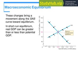
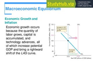
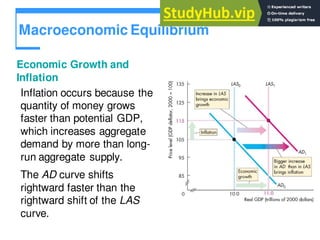
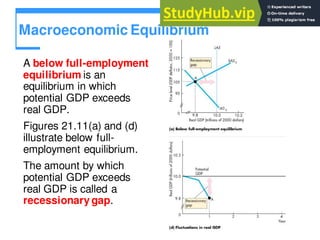
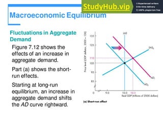
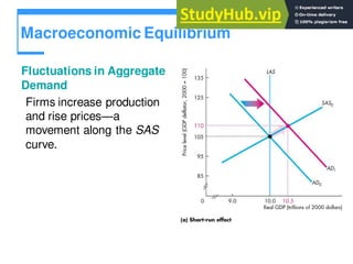
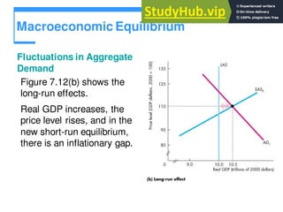
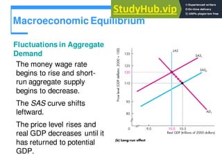
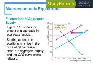
Aggregate demand and aggregate supply determine macroeconomic equilibrium. Aggregate supply depends on labor, capital, and technology and can be either long-run or short-run. Aggregate demand depends on consumption, investment, government spending, and net exports. The intersection of the aggregate demand and supply curves determines equilibrium output and price levels in the short-run. Changes in factors like expectations, fiscal policy, and the world economy cause the aggregate demand curve to shift, affecting equilibrium.

1. AGGREGATE DEMAND
AND
AGGREGATE SUPPLY 7
CHAPTER

2. Objectives
After studying this chapter, you will able to
 Explain what determines aggregate supply
 Explain what determines aggregate demand
 Explain macroeconomic equilibrium
 Explain the effects of changes in aggregate supply and
aggregate demand on economic growth, inflation, and
business cycles
 Explain U.S. economic growth, inflation, and business
cycles by using the AS-AD model.

3. Production and Prices
What forces bring persistent and rapid expansion of real
GDP?
What causes inflation?
Why do we have business cycles?
How do policy actions by the government and the Federal
Reserve affect output and prices?

4. Aggregate Supply
Aggregate Supply Fundamentals
The aggregate quantity of goods and services supplied
depends on three factors:
 The quantity of labor (L )
 The quantity of capital (K )
 The state of technology (T )
The aggregate production function shows how quantity
of real GDP supplied, Y, depends on labor, capital, and
technology.

5. Aggregate Supply
Aggregate Supply Fundamentals
The aggregate production function is written as the
equation:
Y = F(L, K, T ).
In words, the quantity of real GDP supplied depends on (is
a function of) the quantity of labor employed, the quantity
of capital, and the state of technology.
The larger is L, K, or T, the greater is Y.

6. Aggregate Supply
Aggregate Supply Fundamentals
At any given time, the quantity of capital and the state of
technology are fixed but the quantity of labor can vary.
The higher the real wage rate, the smaller is the quantity
of labor demanded and the greater is the quantity of labor
supplied.
The wage rate that makes the quantity of labor demanded
equal to the quantity supplied is the equilibrium wage rate
and at that wage the level of employment is the natural
rate of unemployment.

7. Aggregate Supply
Aggregate Supply Fundamentals
We distinguish two time frames associated with different
states of the labor market:
 Long-run aggregate supply
 Short-run aggregate supply

8. Aggregate Supply
Long-Run Aggregate Supply
The macroeconomic long run is a time frame that is
sufficiently long for all adjustments to be made so that real
GDP equals potential GDP and there is full employment.
The long-run aggregate supply curve (LAS) is the
relationship between the quantity of real GDP supplied
and the price level when real GDP equals potential GDP.

9. Aggregate Supply
Figure 7.1 shows an LAS curve
with potential GDP of $10
trillion.
The LAS curve is vertical
because potential GDP is
independent of the price level.
Along the LAS curve all prices
and wage rates vary by the
same percentage so that
relative prices and the real
wage rate remain constant.

10. Aggregate Supply
Short-Run Aggregate Supply
The macroeconomic short run is a period during which
real GDP has fallen below or risen above potential GDP.
At the same time, the unemployment rate has risen above
or fallen below the natural unemployment rate.
The short-run aggregate supply curve (SAS) is the
relationship between the quantity of real GDP supplied
and the price level in the short-run when the money wage
rate, the prices of other resources, and potential GDP
remain constant.

11. Aggregate Supply
Figure 7.2 shows a short-
run aggregate supply
curve.
Along the SAS curve, rise
in the price level with no
change in the money wage
rate and other input prices
increases the quantity of
real GDP supplied—the
SAS curve is upward
sloping.

12. Aggregate Supply
The SAS curve is upward
sloping because:
A rise in the price level
with no change in costs
induces firms to bear a
higher marginal cost and
increase production.
A fall in the price level with
no change in costs
induces firms to decrease
production to lower
marginal cost.

13. Aggregate Supply
Along the SAS curve, real
GDP might be above
potential GDP…
… or below potential GDP.

14. Aggregate Supply
Movement along the LAS
and SAS Curves
Figure 7.3 summarizes
what you’ve just learned
about the LAS and SAS
curves.
A change in the price level
with an equal percentage
change in the money wage
causes a movement along
the LAS curve.

15. Aggregate Supply
Movement along the LAS
and SAS Curves
Figure 7.3 summarizes
what you’ve just learned
about the LAS and SAS
curves.
A change in the price level
with no change in the
money wage causes a
movement along the SAS
curve.

16. Aggregate Supply
Changes in Aggregate Supply
When potential GDP increases, both the LAS and SAS
curves shift rightward.
Potential GDP changes, for three reasons
 Change in the full-employment quantity of labor.
 Change in the quantity of capital (physical or human).
 Advance in technology.

17. Aggregate Supply
Figure 7.4 shows how
these factors shift the
LAS curve and have
the same effect on the
SAS curve.

18. Aggregate Supply
Figure 7.5 shows the effect
of a change in the money
wage rate on aggregate
supply.
A rise in the money wage
rate decreases short-run
aggregate supply and
shifts the SAS curve
leftward.
But it has no effect on
long-run aggregate supply.

19. Aggregate Demand
The quantity of real GDP demanded, Y, is the total amount
of final goods and services produced in the United States
that people, businesses, governments, and foreigners plan
to buy.
This quantity is the sum of consumption expenditures, C,
investment, I, government purchases, G, and net exports,
X – M. That is:
Y = C + I + G + X – M.

20. Aggregate Demand
Buying plans depend on many factors and some of the
main ones are:
 The price level
 Expectations
 Fiscal and monetary policy
 The world economy

21. Aggregate Demand
The Aggregate Demand Curve
Aggregate demand is the relationship between the
quantity of real GDP demanded and the price level.
The aggregate demand (AD) curve plots the quantity of
real GDP demanded against the price level.

22. Aggregate Demand
Figure 7.6 shows an AD
curve.
The AD curve slopes
downward for two reasons
 A wealth effect
 Substitution effects

23. Aggregate Demand
Wealth effect A rise in the price level, other things
remaining the same, decreases the quantity of real wealth
(money, bonds, stocks, etc.).
To restore their real wealth, people increase saving and
decrease spending, so the quantity of real GDP demanded
decreases.
Similarly, a fall in the price level, other things remaining the
same, increases the quantity of real wealth.
With more real wealth, people decrease saving and
increase spending, so the quantity of real GDP demanded
increases.

24. Aggregate Demand
Intertemporal substitution effect A rise in the price level,
other things remaining the same, decreases the real value
of money and raises the interest rate.
Faced with a higher interest rate, people try to borrow and
spend less so the quantity of real GDP demanded
decreases.
Similarly, a fall in the price level increases the real value of
money and lowers the interest rate.
Faced with a lower interest rate, people borrow and spend
more so the quantity of real GDP demanded increases.

25. Aggregate Demand
International substitution effect A rise in the price level,
other things remaining the same, increases the price of
domestic goods relative to foreign goods, so imports
increase and exports decrease, which decreases the
quantity of real GDP demanded.
Similarly, a fall in the price level, other things remaining
the same, decreases the price of domestic goods relative
to foreign goods, so imports decrease and exports
increase, which increases the quantity of real GDP
demanded.

26. Aggregate Demand
Changes in Aggregate Demand
A change in any influence on buying plans other than the
price level changes aggregate demand.
The main influences on aggregate demand are
 Expectations
 Fiscal and monetary policy
 The world economy.

27. Aggregate Demand
Changes in Aggregate Demand
Expectations about future income, future inflation, and
future profits change aggregate demand.
Increases in expected future income increase people’s
consumption today, and increases aggregate demand.
A rise in the expected inflation rate makes buying goods
cheaper today and increases aggregate demand.
An increase in expected future profits boosts firms’
investment, which increases aggregate demand.

28. Aggregate Demand
Changes in Aggregate Demand
Fiscal policy is the government’s attempt to influence
economic activity by changing its taxes, spending, deficit,
and debt policies.
A tax cut or an increase in transfer payments increases
households’ disposable income—aggregate income
minus taxes plus transfer payments.
An increase in disposable income increases consumption
expenditure and increases aggregate demand.

29. Aggregate Demand
Changes in Aggregate Demand
Because government purchases of goods and services
are one component of aggregate demand, an increase in
government purchases increases aggregate demand.
Monetary policy is changes in the interest rate and
quantity of money.
An increase in the quantity of money increases buying
power and increases aggregate demand.
A cut in the interest rate increases expenditure and
increases aggregate demand.

30. Aggregate Demand
Changes in Aggregate Demand
The world economy influences aggregate demand in two
ways:
A fall in the foreign exchange rate lowers the price of
domestic goods and services relative to foreign goods and
services, increases exports, decreases imports, and
increases aggregate demand.
An increase in foreign income increases the demand for
U.S. exports and increases aggregate demand.

31. Aggregate Demand
Figure 7.7 illustrates
changes in aggregate
demand.
When aggregate demand
increases, the AD curve
shifts rightward…
… and when aggregate
demand decreases, the
AD curve shifts leftward.

32. Macroeconomic Equilibrium
Short-Run Macroeconomic Equilibrium
Short-run macroeconomic equilibrium occurs when the
quantity of real GDP demanded equals the quantity of real
GDP supplied at the point of intersection of the AD curve
and the SAS curve.

33. Macroeconomic Equilibrium
Figure 7.8 illustrates a
short-run equilibrium.
If real GDP is below
equilibrium GDP, firms
increase production and
raise prices…
… and if real GDP is
above equilibrium GDP,
firms decrease production
and lower prices.

34. Macroeconomic Equilibrium
These changes bring a
movement along the SAS
curve toward equilibrium.
In short-run equilibrium,
real GDP can be greater
than or less than potential
GDP.

35. Macroeconomic Equilibrium
Long-Run Macroeconomic Equilibrium
Long-run macroeconomic equilibrium occurs when real
GDP equals potential GDP—when the economy is on its
LAS curve.

36. Macroeconomic Equilibrium
Figure 7.9 illustrates long-
run equilibrium.
Long-run equilibrium
occurs where the AD and
LAS curves intersect and
results when the money
wage has adjusted to put
the SAS curve through the
long-run equilibrium point.

37. Macroeconomic Equilibrium
Economic Growth and
Inflation
Figure 7.10 illustrates
economic growth and
inflation.

38. Macroeconomic Equilibrium
Economic Growth and
Inflation
Economic growth occurs
because the quantity of
labor grows, capital is
accumulated, and
technology advances, all
of which increase potential
GDP and bring a rightward
shift of the LAS curve.

39. Macroeconomic Equilibrium
Economic Growth and
Inflation
Inflation occurs because the
quantity of money grows
faster than potential GDP,
which increases aggregate
demand by more than long-
run aggregate supply.
The AD curve shifts
rightward faster than the
rightward shift of the LAS
curve.

40. Macroeconomic Equilibrium
The Business Cycle
The business cycle occurs because aggregate demand
and the short-run aggregate supply fluctuate but the
money wage does not change rapidly enough to keep real
GDP at potential GDP.

41. Macroeconomic Equilibrium
A below full-employment
equilibrium is an
equilibrium in which
potential GDP exceeds
real GDP.
Figures 21.11(a) and (d)
illustrate below full-
employment equilibrium.
The amount by which
potential GDP exceeds
real GDP is called a
recessionary gap.

42. Macroeconomic Equilibrium
A long-run equilibrium is
an equilibrium in which
potential GDP equals real
GDP.
Figures 21.11(b) and (d)
illustrate long-run
equilibrium.

43. Macroeconomic Equilibrium
An above full-
employment equilibrium
is an equilibrium in which
real GDP exceeds
potential GDP.
Figures 21.11(c) and (d)
illustrate above full-
employment equilibrium.
The amount by which real
GDP exceeds potential
GDP is called an
inflationary gap.

44. Macroeconomic Equilibrium
Figure 7.11(d) shows how,
as the economy moves
from one type of short-run
equilibrium to another, real
GDP fluctuates around
potential GDP in a
business cycle.

45. Macroeconomic Equilibrium
Fluctuations in Aggregate
Demand
Figure 7.12 shows the
effects of an increase in
aggregate demand.
Part (a) shows the short-
run effects.
Starting at long-run
equilibrium, an increase in
aggregate demand shifts
the AD curve rightward.

46. Macroeconomic Equilibrium
Fluctuations in Aggregate
Demand
Firms increase production
and rise prices—a
movement along the SAS
curve.

47. Macroeconomic Equilibrium
Fluctuations in Aggregate
Demand
Figure 7.12(b) shows the
long-run effects.
Real GDP increases, the
price level rises, and in the
new short-run equilibrium,
there is an inflationary gap.

48. Macroeconomic Equilibrium
Fluctuations in Aggregate
Demand
The money wage rate
begins to rise and short-
run aggregate supply
begins to decrease.
The SAS curve shifts
leftward.
The price level rises and
real GDP decreases until it
has returned to potential
GDP.

49. Macroeconomic Equilibrium
Fluctuations in Aggregate
Supply
Figure 7.13 shows the
effects of a decrease in
aggregate supply.
Starting at long-run
equilibrium, a rise in the
price of oil decreases
short-run aggregate supply
and the SAS curve shifts
leftward.

50. Macroeconomic Equilibrium
Fluctuations in Aggregate
Supply
Real GDP decreases and
the price level rises.
The combination of
recession combined with
inflation is called
stagflation.

51. U.S. Economic Growth, Inflation, and
Cycles
Figure 7.14 interprets
the changes in real
GDP and the price
level each year from
1963 to 2003 in
terms of shifting AD,
SAS, and LAS
curves.

52. U.S. Economic Growth, Inflation, and
Cycles
The figure shows the
business cycle,
… long-term
economic growth,…
…. and inflation

53. U.S. Economic Growth, Inflation, and
Cycles
From1963 to 2003:
Real GDP and
potential GDP grew
from $2.8 trillion to
$10.3 trillion.
The price level rose
from 22 to 105.
Business cycle
expansions alternated
with recessions.

54. U.S. Economic Growth, Inflation, and
Cycles
Economic Growth
Real GDP growth was rapid during the 1960s and 1990s
and slower during the 1970s and 1980s.
Inflation
Inflation was the most rapid during the 1970s.
Business Cycles
Recessions occurred during the mid-1970s, 1982, 1991–
1992, and 2001.

55. THE END