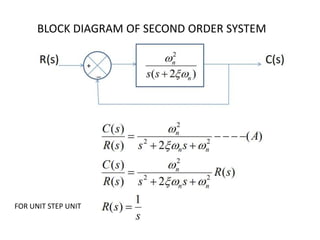
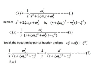
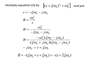
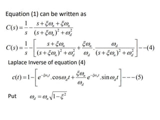
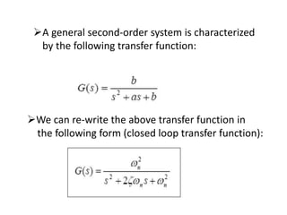
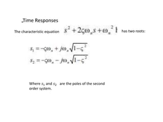
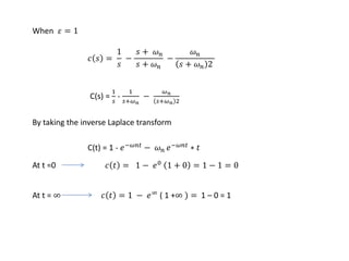
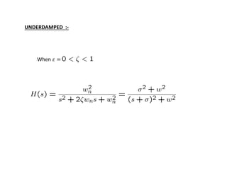
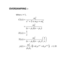
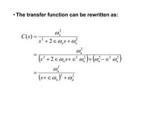
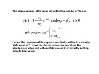
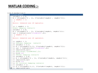
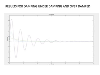
Department of Electrical & Electronics Engineering
Raghu Engineering College (Autonomous)
CASE STUDY
ON
IMPULSE RESPONSE OF SECOND ORDER
SYSTEM
BACHELOR OF TECHNOLOGY
IN
ELECTRICAL AND ELECTRONICS ENGINEERING
Under the Supervision of
Mr.P.SIVA RAMA RAO
Assistant Professor
Mr P.Eswar sai 18981A0237
Mr P.Mohan 18981A0238
Ms P.Supriya 18981A0239
Mr.P.Nitish 18981A0240
Mr.P.Sanjay Kumar 18981A0241
By
Head of the department
Dr.P.SASI KIRAN
Professor
ANALYSIS OF SECOND ORDER SYSTEM
 Damping Ratio : The damping is measured by a factor called as
damping ratio.
 It is denoted by 𝜀 .
 So when zeta is maximum ; it produces maximum opposition to the
oscillatory behaviour of system.
BLOCK DIAGRAM OF SECOND ORDER SYSTEM
FOR UNIT STEP UNIT
A general second-order system is characterized
by the following transfer function:
We can re-write the above transfer function in
the following form (closed loop transfer function):
 According the value of ζ, a second-order system can be
set into one of the four categories:
1. OVER DAMPED : when the system has two real distinct poles (𝜖 >1).
2. UNDER DAMPED :
when the system has two complex conjugate
poles (0 <𝜖 <1)
3. UN-DAMPED : when the system has two imaginary poles (𝜖 = 0).
4. CRITICALLY DAMPED :
when the system has two real but equal poles
(𝜖 = 1).
IMPULSE RESPONSE OF THE SECOND ORDER SYSTEM:
„Laplace transform of the unit impulse is R(s)=1
„Impulse response :-
„Transient response for the impulse function, which is simply is the derivative
of the response to the unit step: derivative of the response to the unit step:
„Time Responses
The characteristic equation has two roots:
Where 𝑠1 and 𝑠2 are the poles of the second
order system.
𝑐 𝑠 =
1
𝑠
−
𝑠 + 𝜔 𝑛
𝑠 + 𝜔 𝑛
−
𝜔 𝑛
𝑠 + 𝜔 𝑛 2
When 𝜀 = 1
C(s) =
1
𝑠
-
1
𝑠+𝜔 𝑛
−
𝜔 𝑛
𝑠+𝜔 𝑛 2
By taking the inverse Laplace transform
C(t) = 1 - 𝑒−𝜔𝑛𝑡
− 𝜔 𝑛 𝑒−𝜔𝑛𝑡
∗ 𝑡
At t =0 𝑐 𝑡 = 1 − 𝑒0
1 + 0 = 1 − 1 = 0
At t = ∞ 𝑐 𝑡 = 1 − 𝑒∞ ( 1 +∞ ) = 1 – 0 = 1
When 𝜀 =
UNDERDAMPED :-
When 𝜀 > 1,
OVERDAMPING :-
  0,1)(
1
))((
)(
1
)(
))((
2
)(
21
11
21
2
21
2
21
2
22
2














tekek
pp
ty
spsps
sY
s
sX
psps
ss
sC
tptpn
n
n
nn
n





• The transfer function can be rewritten as:
   
  22
2
222222
2
22
2
2
2
)(
dn
n
nnnn
n
nn
n
s
ss
ss
sC












• The step response, after some simplification, can be written as:
• Hence, the response of this system eventually settles to a steady-
state value of 1. However, the response can overshoot the
steady-state value and will oscillate around it, eventually settling
in to its final value.
 











n
d
d
t
n
n
where
ttety n





 
1
tan
0,sin1)(
IMPULSE RESPONSE:
The first pulse has a width T and height 1/T, area of the pulse will be 1. If we halve
the duration and double the amplitude we get second pulse. The area under the
second pulse is also unity
The pulse for which the duration tends to zero and amplitude tends to infinity is
called impulse. Impulse function also known as delta function.
MATLAB CODING :-
RESULTS FOR DAMPING UNDER DAMPING AND OVER DAMPED
REFERENCES :-
1. AUTOMATIC CONTROL SYSTEM KUO & GOLNARAGHI
2. 2. CONTROL SYSTEM ANAND KUMAR
3. 3. AUTOMATIC CONTROL SYSTEM
4. CLASS NOTES
IMPULSE RESPONSE OF SECOND ORDER SYSTEM

IMPULSE RESPONSE OF SECOND ORDER SYSTEM

  • 1.
    Department of Electrical& Electronics Engineering Raghu Engineering College (Autonomous) CASE STUDY ON IMPULSE RESPONSE OF SECOND ORDER SYSTEM BACHELOR OF TECHNOLOGY IN ELECTRICAL AND ELECTRONICS ENGINEERING Under the Supervision of Mr.P.SIVA RAMA RAO Assistant Professor Mr P.Eswar sai 18981A0237 Mr P.Mohan 18981A0238 Ms P.Supriya 18981A0239 Mr.P.Nitish 18981A0240 Mr.P.Sanjay Kumar 18981A0241 By Head of the department Dr.P.SASI KIRAN Professor
  • 2.
    ANALYSIS OF SECONDORDER SYSTEM  Damping Ratio : The damping is measured by a factor called as damping ratio.  It is denoted by 𝜀 .  So when zeta is maximum ; it produces maximum opposition to the oscillatory behaviour of system.
  • 3.
    BLOCK DIAGRAM OFSECOND ORDER SYSTEM FOR UNIT STEP UNIT
  • 19.
    A general second-ordersystem is characterized by the following transfer function: We can re-write the above transfer function in the following form (closed loop transfer function):
  • 20.
     According thevalue of ζ, a second-order system can be set into one of the four categories: 1. OVER DAMPED : when the system has two real distinct poles (𝜖 >1). 2. UNDER DAMPED : when the system has two complex conjugate poles (0 <𝜖 <1) 3. UN-DAMPED : when the system has two imaginary poles (𝜖 = 0). 4. CRITICALLY DAMPED : when the system has two real but equal poles (𝜖 = 1).
  • 21.
    IMPULSE RESPONSE OFTHE SECOND ORDER SYSTEM: „Laplace transform of the unit impulse is R(s)=1 „Impulse response :- „Transient response for the impulse function, which is simply is the derivative of the response to the unit step: derivative of the response to the unit step:
  • 22.
    „Time Responses The characteristicequation has two roots: Where 𝑠1 and 𝑠2 are the poles of the second order system.
  • 23.
    𝑐 𝑠 = 1 𝑠 − 𝑠+ 𝜔 𝑛 𝑠 + 𝜔 𝑛 − 𝜔 𝑛 𝑠 + 𝜔 𝑛 2 When 𝜀 = 1 C(s) = 1 𝑠 - 1 𝑠+𝜔 𝑛 − 𝜔 𝑛 𝑠+𝜔 𝑛 2 By taking the inverse Laplace transform C(t) = 1 - 𝑒−𝜔𝑛𝑡 − 𝜔 𝑛 𝑒−𝜔𝑛𝑡 ∗ 𝑡 At t =0 𝑐 𝑡 = 1 − 𝑒0 1 + 0 = 1 − 1 = 0 At t = ∞ 𝑐 𝑡 = 1 − 𝑒∞ ( 1 +∞ ) = 1 – 0 = 1
  • 24.
  • 25.
    When 𝜀 >1, OVERDAMPING :-   0,1)( 1 ))(( )( 1 )( ))(( 2 )( 21 11 21 2 21 2 21 2 22 2               tekek pp ty spsps sY s sX psps ss sC tptpn n n nn n     
  • 26.
    • The transferfunction can be rewritten as:       22 2 222222 2 22 2 2 2 )( dn n nnnn n nn n s ss ss sC            
  • 27.
    • The stepresponse, after some simplification, can be written as: • Hence, the response of this system eventually settles to a steady- state value of 1. However, the response can overshoot the steady-state value and will oscillate around it, eventually settling in to its final value.              n d d t n n where ttety n        1 tan 0,sin1)(
  • 28.
    IMPULSE RESPONSE: The firstpulse has a width T and height 1/T, area of the pulse will be 1. If we halve the duration and double the amplitude we get second pulse. The area under the second pulse is also unity The pulse for which the duration tends to zero and amplitude tends to infinity is called impulse. Impulse function also known as delta function.
  • 29.
  • 30.
    RESULTS FOR DAMPINGUNDER DAMPING AND OVER DAMPED
  • 31.
    REFERENCES :- 1. AUTOMATICCONTROL SYSTEM KUO & GOLNARAGHI 2. 2. CONTROL SYSTEM ANAND KUMAR 3. 3. AUTOMATIC CONTROL SYSTEM 4. CLASS NOTES