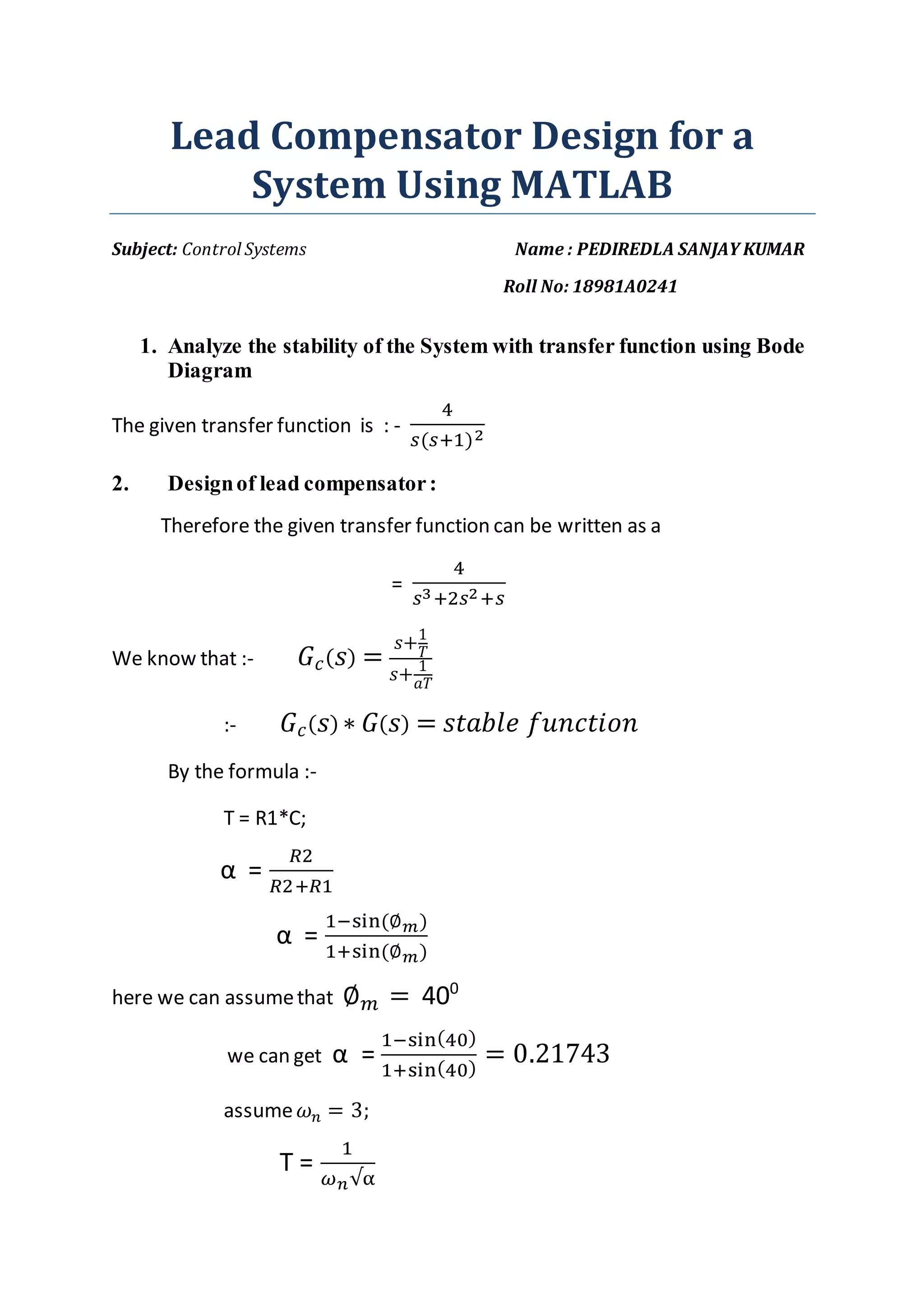
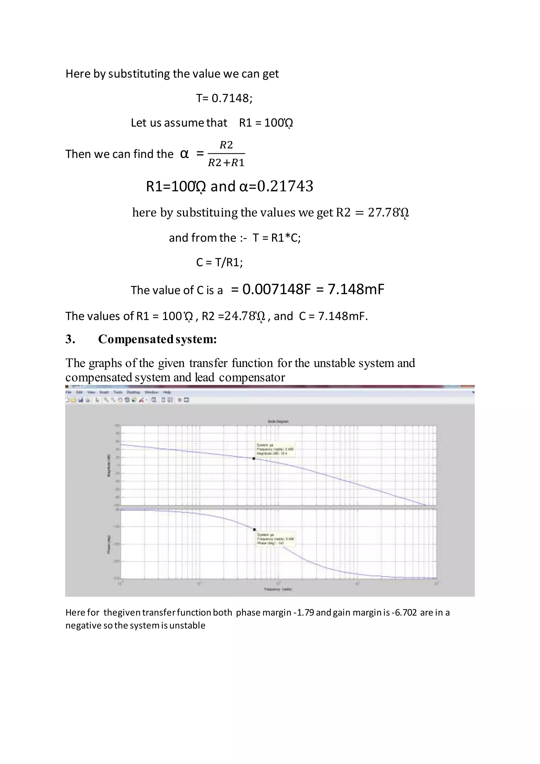
The document discusses the design of a lead compensator for a control system using MATLAB, focusing on stability analysis through Bode diagrams. Initial calculations reveal instability with negative phase and gain margins, but after compensation, both margins become positive, indicating system stability. Key parameters such as resistances and capacitance values are also derived in the document.

1. Lead Compensator Design for a
System Using MATLAB
Subject: Control Systems Name : PEDIREDLA SANJAY KUMAR
Roll No: 18981A0241
1. Analyze the stability of the System with transfer function using Bode
Diagram
The given transfer function is : -
4
𝑠(𝑠+1)2
2. Designof lead compensator:
Therefore the given transfer function can be written as a
=
4
𝑠3+2𝑠2+𝑠
We know that :- 𝐺 𝑐( 𝑠) =
𝑠+1
𝑇
𝑠+ 1
𝑎𝑇
:- 𝐺 𝑐( 𝑠) ∗ 𝐺( 𝑠) = 𝑠𝑡𝑎𝑏𝑙𝑒 𝑓𝑢𝑛𝑐𝑡𝑖𝑜𝑛
By the formula :-
T = R1*C;
α =
𝑅2
𝑅2+𝑅1
α =
1−sin(∅ 𝑚)
1+sin(∅ 𝑚)
here we can assumethat ∅ 𝑚 = 400
we can get α =
1−sin(40)
1+sin(40)
= 0.21743
assume 𝜔 𝑛 = 3;
T =
1
𝜔 𝑛√α

2. Here by substituting the value we can get
T= 0.7148;
Let us assumethat R1 = 100ᾩ
Then we can find the α =
𝑅2
𝑅2+𝑅1
R1=100ᾩ and α=0.21743
here by substituing the values we get R2 = 27.78ᾩ
and fromthe :- T = R1*C;
C = T/R1;
The value of C is a = 0.007148F = 7.148mF
The values of R1 = 100 ᾩ , R2 =24.78ᾩ , and C = 7.148mF.
3. Compensatedsystem:
The graphs of the given transfer function for the unstable system and
compensated system and lead compensator
Here for thegiventransferfunctionboth phase margin -1.79 andgain marginis -6.702 are in a
negative sothe systemisunstable

3. This is for the lead compensated system
This is the plotting for after adding compensatorto the system and now the
gain margin Is the 3.97 and the phase margin is the 8.23.since both the gain
margin and phase margin are positive so the system is stable.

4. 4. Any other observations:
The matlab codeis given below :-