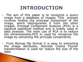
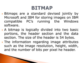
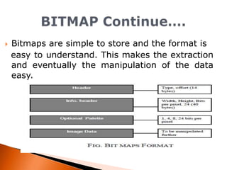
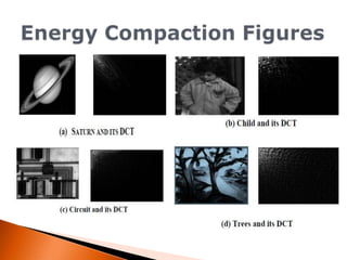
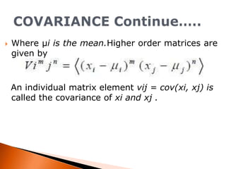
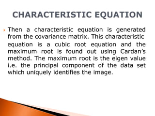
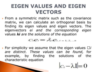
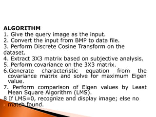
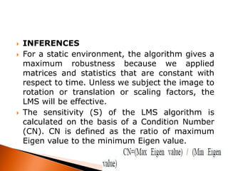
1.
2.
3.
4.
5.

6.
7.
8.

INTRODUCTION
BITMAP
DISCRETE COSINE TRANSFORMATION
ENERGY COMPACTION
CHARACTERSTICS EQUATIONS
EIGEN VALUE & EIGEN VECTOR
LEAST MEANS SQURE EQUATION
CONCLSION




The aim of this paper is to recognize a query
image from a database of images. This process
involves finding the principal component of the
image, which distinguishes it from the other
images. Principal Component Analysis (PCA) is a
classical statistical method and is widely used in
data analysis. The main use of PCA is to reduce
the dimensionality.PCS Is used for recognize the
image by extracting the principle components.
From Bitmap file format it is easy to extracting
the image attributes. Discrete Cosine Fourier
transformation is used for reduce the size of the
data.






Bitmaps are a standard devised jointly by
Microsoft and IBM for storing images on IBM
compatible PC’s running the Windows
software.
A bitmap is logically divided into two basic
portions, the header section and the data
section. The size of the header is 54 bytes.
The information regarding image attributes
such as the image resolution, height, width,
and the number of bits per pixel he header.


Bitmaps are simple to store and the format is
easy to understand. This makes the extraction
and eventually the manipulation of the data
easy.







Several algorithms may be used for the
recognition
process.
Some
of
them
are
Multidimensional
Scaling,
Singular
Value
Decomposition (SVD) and Factor analysis (FA).
MDS provides a visual representation of the
patterns of proximities in the data set. It is
applied on a matrix containing distance measures
between the variables of the data set.
SVD can be applied only to singular matrices. It
attempts to represent a singular matrix.
Factor analysis aims to highlight the variances
amongst a large number of observable data
through a set of unobservable data called factors.
FA can be approached in two ways. They are
a) Principal Component Analysis
b) Common Factor Analysis.






Common factor analysis(CFA) considers the
common variances of the variables concerned. It
results in a testable model that explains
intercorrelations amongst the variables.
Principal Component Analysis (PCA) considers
the total variance of the data set. Hence given an
image input, PCA would summarize the total
variance in image values.
Advantage of PCA is It can accept both
subjective and objective attributes and always
results in a unique solution.







Transform coding constitutes an integral component
of
contemporary
image/video
processing
applications.
Some properties of the DCT, which are of particular
value to image processing applications:
De correlation: The principle advantage of image
transformation is the removal of redundancy
between neighbouring pixels. This property helps us
to
manipulate
the
uncorrelated
transform
coefficients as they can be operated upon
independently.
Energy Compaction: This property can be
explained by using a few examples given below with
figs..






The example comprises of four broad image
classes. Figure (a) and (b) contain large areas of
slowly varying intensities. These images can be
classified as low frequency images with low spatial
details.
Figure (c) contains a number of edges (i.e., sharp
intensity variations) and therefore can be
classified as a high frequency image with low
spatial content.
Figure (d) However, the image data exhibits high
correlation, which is exploited by the DCT
algorithm to provide good energy compaction






The general equation for a 2D (N by M image) DCT is
defined by the following equation:

The good performance shown by 2D DCT with PCA
method is direct result of coupling 2D DCT coefficients
with PCA method. It mainly benefits from using 2D
discrete cosine transform to eliminate the correlation
between rows and columns and get energy
concentrated at the same
time.




Covariance is a property that gives us the
amount of variation of two dimensions from
their mean with respect to each other. This
property is used on the DCT-matrix so that a
form of distance measure is performed on the
image pixel values thus providing their relative
intensity measures.
The covariance of two variants Xi And Xj and
provides a measure of how strongly correlated
these variables are, and the derived quantity.


where σi , σj are the standard deviations, is
called statistical Correlation of xi and xj . The
covariance is symmetric since
cov (x, y)
= cov ( y, x) Covariance is performed on the
extracted 3*3 DCT matrix and covariance
matrix is calculated using the following
formulae Given n sets of variants denoted
{x1},.....,{xn}, the first-order covariance
matrix is defined by


Where µi is the mean.Higher order matrices are
given by

An individual matrix element vij = cov(xi, xj) is
called the covariance of xi and xj .


Then a characteristic equation is generated
from the covariance matrix. This characteristic
equation is a cubic root equation and the
maximum root is found out using Cardan’s
method. The maximum root is the eigen value
i.e. the principal component of the data set
which uniquely identifies the image.




From a symmetric matrix such as the covariance
matrix, we can calculate an orthogonal basis by
finding its eigen values and eigen vectors. The
eigenvectors ei and the corresponding eigen
values λi are the solutions of the equation

For simplicity we assume that the eigen values i
are distinct. These values can be found, for
example, by finding the solutions of the
characteristic equation







where the I is the identity matrix having the same
order than Cx and the |.| denotes the determinant
of the matrix. We are here faced with contradictory
goals:
1. On one hand, we should simplify the problem by
reducing the dimension of the representation.
2. On the other hand we want to preserve as much
as possible of the original information content.
PCA offers a convenient way to control the trade off
between loosing information and simplifying the
problem at hand.








The database of images is a collection of the Eigen
vectors of the different images that correspond to
the maximum Eigen value.
The Eigen vectors play an important role in the
image recognition process. We need to define
stepwise rules that need to be executed to achieve
image recognition.
There are basically two kinds of environments
classified based on the adaptation nature. They are
described below:
1. Static Environment : The system is said to be
static in nature if there is a negative output for a
new image given as a input. The system responds
negatively even when a existing image in the
database is rotated or translated or is subjected to
changes in contrast, brightness, scaling factors etc.




2. Dynamic Environment: The system is said
to be dynamic in nature if there exists a
learning process if any image is fed for the
recognition process.
Least Mean Square Algorithm:
Generally, LMS algorithm is implemented using
the instantaneous values for the input function.
The name itself defines the rough formula, as
LMS is a least value of the squares of the
means calculated with respect to a maximum
Eigen value calculated for a particular Eigen
space. The major property of LMS algorithm is
that it operates linearly.




Advantages of LMS algorithm: The
reasons of adopting LMS in our paper are
due
to
its
properties
like
Model
independence, Robustness, Optimality in
results and Simplicity.
LMS formula: After we defined a
general formula, as we adopted a
statistical and matrices concepts, we
necessarily define a specific formula as
follows:
ALGORITHM
1. Give the query image as the input.
2. Convert the input from BMP to data file.
3. Perform Discrete Cosine Transform on the
dataset.
4. Extract 3X3 matrix based on subjective analysis.
5. Perform covariance on the 3X3 matrix.
6.Generate characteristic equation from the
covariance matrix and solve for maximum Eigen
value.
7. Perform comparison of Eigen values by Least
Mean Square Algorithm (LMS).
8 If LMS=0, recognize and display image; else no
 match found.





INFERENCES
For a static environment, the algorithm gives a
maximum robustness because we applied
matrices and statistics that are constant with
respect to time. Unless we subject the image to
rotation or translation or scaling factors, the
LMS will be effective.
The sensitivity (S) of the LMS algorithm is
calculated on the basis of a Condition Number
(CN). CN is defined as the ratio of maximum
Eigen value to the minimum Eigen value.






This
paper
finds
immense
applications
pertaining to security aspects in government
agencies and public places with economical
software implementation. Though such a
system may prove to be an asset for security
purposes it fails when the application involves
the classification and categorization of images
based on their content.
Secondly, an image whose brightness or
contrast has been changed from the original,
though present in the database will not be
recognized by the system.
The use of bitmapped images results in the
occupation of a significant amount of memory.
Image recogonization

Image recogonization

  • 2.
    1. 2. 3. 4. 5. 6. 7. 8. INTRODUCTION BITMAP DISCRETE COSINE TRANSFORMATION ENERGYCOMPACTION CHARACTERSTICS EQUATIONS EIGEN VALUE & EIGEN VECTOR LEAST MEANS SQURE EQUATION CONCLSION
  • 3.
      The aim ofthis paper is to recognize a query image from a database of images. This process involves finding the principal component of the image, which distinguishes it from the other images. Principal Component Analysis (PCA) is a classical statistical method and is widely used in data analysis. The main use of PCA is to reduce the dimensionality.PCS Is used for recognize the image by extracting the principle components. From Bitmap file format it is easy to extracting the image attributes. Discrete Cosine Fourier transformation is used for reduce the size of the data.
  • 4.
       Bitmaps are astandard devised jointly by Microsoft and IBM for storing images on IBM compatible PC’s running the Windows software. A bitmap is logically divided into two basic portions, the header section and the data section. The size of the header is 54 bytes. The information regarding image attributes such as the image resolution, height, width, and the number of bits per pixel he header.
  • 5.
     Bitmaps are simpleto store and the format is easy to understand. This makes the extraction and eventually the manipulation of the data easy.
  • 6.
        Several algorithms maybe used for the recognition process. Some of them are Multidimensional Scaling, Singular Value Decomposition (SVD) and Factor analysis (FA). MDS provides a visual representation of the patterns of proximities in the data set. It is applied on a matrix containing distance measures between the variables of the data set. SVD can be applied only to singular matrices. It attempts to represent a singular matrix. Factor analysis aims to highlight the variances amongst a large number of observable data through a set of unobservable data called factors. FA can be approached in two ways. They are a) Principal Component Analysis b) Common Factor Analysis.
  • 7.
       Common factor analysis(CFA)considers the common variances of the variables concerned. It results in a testable model that explains intercorrelations amongst the variables. Principal Component Analysis (PCA) considers the total variance of the data set. Hence given an image input, PCA would summarize the total variance in image values. Advantage of PCA is It can accept both subjective and objective attributes and always results in a unique solution.
  • 8.
        Transform coding constitutesan integral component of contemporary image/video processing applications. Some properties of the DCT, which are of particular value to image processing applications: De correlation: The principle advantage of image transformation is the removal of redundancy between neighbouring pixels. This property helps us to manipulate the uncorrelated transform coefficients as they can be operated upon independently. Energy Compaction: This property can be explained by using a few examples given below with figs..
  • 10.
       The example comprisesof four broad image classes. Figure (a) and (b) contain large areas of slowly varying intensities. These images can be classified as low frequency images with low spatial details. Figure (c) contains a number of edges (i.e., sharp intensity variations) and therefore can be classified as a high frequency image with low spatial content. Figure (d) However, the image data exhibits high correlation, which is exploited by the DCT algorithm to provide good energy compaction
  • 11.
       The general equationfor a 2D (N by M image) DCT is defined by the following equation: The good performance shown by 2D DCT with PCA method is direct result of coupling 2D DCT coefficients with PCA method. It mainly benefits from using 2D discrete cosine transform to eliminate the correlation between rows and columns and get energy concentrated at the same time.
  • 12.
      Covariance is aproperty that gives us the amount of variation of two dimensions from their mean with respect to each other. This property is used on the DCT-matrix so that a form of distance measure is performed on the image pixel values thus providing their relative intensity measures. The covariance of two variants Xi And Xj and provides a measure of how strongly correlated these variables are, and the derived quantity.
  • 13.
     where σi ,σj are the standard deviations, is called statistical Correlation of xi and xj . The covariance is symmetric since cov (x, y) = cov ( y, x) Covariance is performed on the extracted 3*3 DCT matrix and covariance matrix is calculated using the following formulae Given n sets of variants denoted {x1},.....,{xn}, the first-order covariance matrix is defined by
  • 14.
     Where µi isthe mean.Higher order matrices are given by An individual matrix element vij = cov(xi, xj) is called the covariance of xi and xj .
  • 15.
     Then a characteristicequation is generated from the covariance matrix. This characteristic equation is a cubic root equation and the maximum root is found out using Cardan’s method. The maximum root is the eigen value i.e. the principal component of the data set which uniquely identifies the image.
  • 16.
      From a symmetricmatrix such as the covariance matrix, we can calculate an orthogonal basis by finding its eigen values and eigen vectors. The eigenvectors ei and the corresponding eigen values λi are the solutions of the equation For simplicity we assume that the eigen values i are distinct. These values can be found, for example, by finding the solutions of the characteristic equation
  • 17.
        where the Iis the identity matrix having the same order than Cx and the |.| denotes the determinant of the matrix. We are here faced with contradictory goals: 1. On one hand, we should simplify the problem by reducing the dimension of the representation. 2. On the other hand we want to preserve as much as possible of the original information content. PCA offers a convenient way to control the trade off between loosing information and simplifying the problem at hand.
  • 18.
        The database ofimages is a collection of the Eigen vectors of the different images that correspond to the maximum Eigen value. The Eigen vectors play an important role in the image recognition process. We need to define stepwise rules that need to be executed to achieve image recognition. There are basically two kinds of environments classified based on the adaptation nature. They are described below: 1. Static Environment : The system is said to be static in nature if there is a negative output for a new image given as a input. The system responds negatively even when a existing image in the database is rotated or translated or is subjected to changes in contrast, brightness, scaling factors etc.
  • 19.
      2. Dynamic Environment:The system is said to be dynamic in nature if there exists a learning process if any image is fed for the recognition process. Least Mean Square Algorithm: Generally, LMS algorithm is implemented using the instantaneous values for the input function. The name itself defines the rough formula, as LMS is a least value of the squares of the means calculated with respect to a maximum Eigen value calculated for a particular Eigen space. The major property of LMS algorithm is that it operates linearly.
  • 20.
      Advantages of LMSalgorithm: The reasons of adopting LMS in our paper are due to its properties like Model independence, Robustness, Optimality in results and Simplicity. LMS formula: After we defined a general formula, as we adopted a statistical and matrices concepts, we necessarily define a specific formula as follows:
  • 22.
    ALGORITHM 1. Give thequery image as the input. 2. Convert the input from BMP to data file. 3. Perform Discrete Cosine Transform on the dataset. 4. Extract 3X3 matrix based on subjective analysis. 5. Perform covariance on the 3X3 matrix. 6.Generate characteristic equation from the covariance matrix and solve for maximum Eigen value. 7. Perform comparison of Eigen values by Least Mean Square Algorithm (LMS). 8 If LMS=0, recognize and display image; else no  match found.
  • 23.
       INFERENCES For a staticenvironment, the algorithm gives a maximum robustness because we applied matrices and statistics that are constant with respect to time. Unless we subject the image to rotation or translation or scaling factors, the LMS will be effective. The sensitivity (S) of the LMS algorithm is calculated on the basis of a Condition Number (CN). CN is defined as the ratio of maximum Eigen value to the minimum Eigen value.
  • 24.
       This paper finds immense applications pertaining to securityaspects in government agencies and public places with economical software implementation. Though such a system may prove to be an asset for security purposes it fails when the application involves the classification and categorization of images based on their content. Secondly, an image whose brightness or contrast has been changed from the original, though present in the database will not be recognized by the system. The use of bitmapped images results in the occupation of a significant amount of memory.