Feature Extraction
Featureextraction is a machine learning and data analysis process that
transforms raw data into numerical features.
Feature extraction refers to the process of transforming raw data into
numerical features that can be processed while preserving the information in
the original data set.
Feature extraction is a process used in machine learning to reduce the
number of resources needed for processing without losing important or
relevant information.
3.
Why is FeatureExtraction Important?
Reduction of Computational Cost: By reducing the dimensionality of the data,
machine learning algorithms can run more quickly.
Improved Performance: Algorithms often perform better with a reduced number of
features. This is because noise and irrelevant details are removed, allowing the
algorithm to focus on the most important aspects of the data.
Prevention of Overfitting: With too many features, models can become overfitted to
the training data, meaning they may not generalize well to new, unseen data. Feature
extraction helps to prevent this by simplifying the model.
Better Understanding of Data: Extracting and selecting important features can
provide insights into the underlying processes that generated the data.
4.
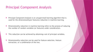
Principal Component Analysis
Principal Component Analysis is an unsupervised learning algorithm that is
used for the dimensionality(or features) reduction in machine learning.
Dimensionality reduction in machine learning refers to the process of reducing
the number of random variables (or features) under consideration.
This reduction can be achieved by obtaining a set of principal variables.
Dimensionality reduction can be used for feature selection, feature
extraction, or a combination of the two.
5.
Principal ComponentAnalysis (PCA) is an unsupervised learning algorithm
technique used to examine the interrelations among a set of variables. It is
also known as a general factor analysis
6.
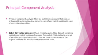
Principal Component Analysis
Principal Component Analysis (PCA) is a statistical procedure that uses an
orthogonal transformation that converts a set of correlated variables to a set
of uncorrelated variables.
Set of Correlated Variables: PCA is typically applied to a dataset containing
multiple correlated variables (features). The goal of PCA is to find a new set
of variables (principal components) that are linear combinations of the
original variables but are uncorrelated with each other.
7.
Uncorrelated Variables:The principal components derived from PCA are
uncorrelated, which means that the covariance between any pair of principal
components is zero.
8.
The PCAalgorithm is based on some mathematical concepts such as:
• Variance and Covariance
• Eigenvalues and Eigen vectors
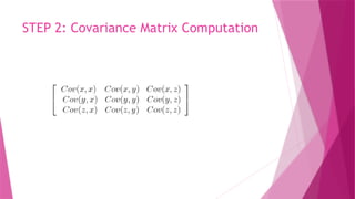
Step 3: ComputeEigenvalues and Eigenvectors of
Covariance Matrix to Identify Principal Components
14.
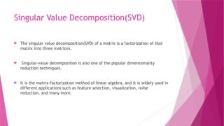
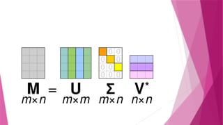
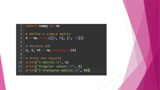
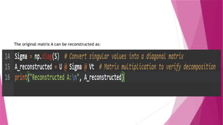
Singular Value Decomposition(SVD)
The singular value decomposition(SVD) of a matrix is a factorization of that
matrix into three matrices.
Singular-value decomposition is also one of the popular dimensionality
reduction techniques.
It is the matrix-factorization method of linear algebra, and it is widely used in
different applications such as feature selection, visualization, noise
reduction, and many more.
17.
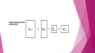
U isan × orthogonal matrix (columns are left singular vectors).
𝑚 𝑚
Σ is an × diagonal matrix (singular values).
𝑚 𝑛
𝑉𝑇
is an × orthogonal matrix (rows of
𝑛 𝑛 𝑉𝑇
are right singular vectors).
Intensity Levelof the image(Which is applicable in Discrete signal)
Since an image is contiguous, the values of most pixels depend on the pixels
around them.
Feature Selection
Featureselection retains the most relevant features from the existing
ones and removes irrelevant or redundant features.
While developing the machine learning model, only a few variables in
the dataset are useful for building the model, and the rest features
are either redundant or irrelevant.
If we input the dataset with all these redundant and irrelevant
features, it may negatively impact and reduce the overall
performance and accuracy of the model.
24.
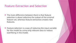
Feature Extraction andSelection
The main difference between them is that feature
selection is about selecting the subset of the original
feature set, whereas feature extraction creates new
features.
Feature selection is a way of reducing the input variable
for the model by using only relevant data to reduce
overfitting in the model.
25.
Need for FeatureSelection
Before implementing any technique, it is really important to
understand, need for the technique and so for the Feature Selection.
As we know, in machine learning, it is necessary to provide a pre-
processed and good input dataset in order to get better outcomes.
We collect a huge amount of data to train our model and help it to
learn better. Generally, the dataset consists of noisy data, irrelevant
data, and some part of useful data. Moreover, the huge amount of
data also slows down the training process of the model, and with
noise and irrelevant data, the model may not predict and perform
well.
26.
Benefits of usingfeature selection in
machine learning:
• It helps in avoiding the curse of dimensionality.
• It helps in the simplification of the model so that it can be easily
interpreted by the researchers.
• It reduces the training time.
• It reduces overfitting hence enhance the generalization.
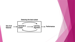
Wrapper Method
Inwrapper methods, different subsets of features are
evaluated by training a model for each subset, and then
the performance is compared and the right
combination is chosen.
Forward Selection
• Startingfrom Scratch: Begin with an empty set of features and iteratively
add one feature at a time.
• Model Evaluation: At each step, train and evaluate the machine learning
model using the selected features.
• Stopping Criterion: Continue until a predefined stopping criterion is met,
such as a maximum number of features or a significant drop in
performance.
32.
Backward Elimination
• Startingwith Everything: Start with all available features.
• Iterative Removal: In each iteration, remove the least important feature
and evaluate the model.
• Stopping Criterion: Continue until a stopping condition is met.
33.
Exhaustive Feature Selection
•Exploring All Possibilities: Evaluate all possible combinations of features,
which ensures finding the best subset for model performance.
• Computational Cost: This can be computationally expensive, especially
with a large number of features.
34.
Recursive Feature Elimination(RFE)
• Ranking Features: Start with all features and rank them based on their
importance or contribution to the model.
• Iterative Removal: In each iteration, remove the least important
feature(s).
• Stopping Criterion: Continue until a desired number of features is
reached.
35.
Filter Method
Thesemethods are generally used while doing the pre-processing step.
These methods select features from the dataset irrespective of the use of
any machine learning algorithm.
In terms of computation, they are very fast and inexpensive and are very
good for removing duplicated, correlated, redundant features but these
methods do not remove multicollinearity.
Information Gain
Itis defined as the amount of information provided by the feature for
identifying the target value and measures reduction in the entropy values.
Information gain of each attribute is calculated considering the target values
for feature selection.
39.
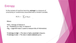
Entropy
Where:
•H(X) = Entropyof feature X
•pi= Probability of class i in feature X
•log2= Logarithm base 2 (used to measure bits of information)
•If entropy is high The data is highly
→ uncertain (impure).
•If entropy is low The data is
→ more ordered (pure).
In the context of machine learning, entropy is a measure of
uncertainty or randomness associated with a random variable.
40.
Chi-square test
Chi-squaremethod (X2
) is generally used to test the relationship between
categorical variables. It compares the observed values from different
attributes of the dataset to its expected value.
41.
Fisher’s Score
Fisher’sScore selects each feature independently according to their scores
under Fisher criterion leading to a suboptimal set of features. The larger the
Fisher’s score is, the better is the selected feature.
Higher Fisher Score More important feature
→
Lower Fisher Score Less relevant feature
→
42.
Fisher’s Score
Where:
•Nc =Number of samples in class c.
•μc = Mean of feature xjin class c.
•μ = Overall mean of feature xjacross all classes.
•σc
2
= Variance of feature xjin class c.
43.
Correlation Coefficient
Pearson’sCorrelation Coefficient is a measure of quantifying the association
between the two continuous variables and the direction of the relationship
with its values ranging from -1 to 1.
Xi= Individual values of feature X
Yi= Individual values of feature Y
Xˉ = Mean (average) of feature X
Yˉ = Mean (average) of feature Y
44.
Embedded Method
Embeddedmethods combine the advantageous aspects of both Filter and
Wrapper methods.
Embedded methods combined the advantages of both filter and wrapper
methods by considering the interaction of features along with low
computational cost.
These are fast processing methods similar to the filter method but more
accurate than the filter method.
46.
These methodsare also iterative, which evaluates each iteration, and
optimally finds the most important features that contribute the most to
training in a particular iteration.
47.
Some techniques ofembedded methods
Regularization
Random Forest Importance
48.
Regularization
Regularization addsa penalty term to different parameters of the machine
learning model to avoid overfitting in the model.
This penalty term is added to the coefficients; hence it shrinks some
coefficients to zero. Those features with zero coefficients can be removed from
the dataset.
The types of regularization techniques are L1 Regularization (Lasso
Regularization) or d L2 regularization(Ridge Regularization)
Uses L1 penalty, which shrinks less important features to zero, effectively
removing them.
Uses L2 penalty, which reduces feature weights but does not remove them
completely.
49.
Random Forest Importance
Different tree-based methods of feature selection help us with feature
importance to provide a way of selecting features. Here, feature
importance specifies which feature has more importance in model building
or has a great impact on the target variable.
Random Forest is a tree-based method, which is a type of bagging
algorithm that aggregates a different number of decision trees.
50.
Evaluating ML Algoand Model Selection
Model evaluation is the process that uses some metrics that help us to
analyze the performance of the model.
51.
Accuracy
Accuracy: Accuracyis defined as the ratio of the number of correct
predictions to the total number of predictions.
accuracy_score
from sklearn.metrics import accuracy_score
# Actual labels
y_true = [0, 1, 1, 0, 1, 0, 1, 1]
# Predicted labels
y_pred = [0, 1, 0, 0, 1, 1, 1, 1]
# Calculate accuracy
accuracy = accuracy_score(y_true, y_pred)
print(f"Accuracy: {accuracy * 100:.2f}%")
52.
Precision
Precision isthe ratio of true positives to the summation of true positives
and false positives. It basically analyses the positive predictions.
The drawback of Precision is that it does not consider the True Negatives
and False Negatives.
precision_score()
53.
Recall
Recall isthe ratio of true positives to the summation of true positives and
false negatives. It basically analyses the number of correct positive
samples.
recall_score()
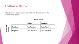
Explanation
True Positive:- This is the number of times the model predicted an
independent variable as positive when the actual value was positive.
False Positive: - This is the number of times the model predicted an
independent variable as positive when the actual value was negative.
False Negative: - This is the number of times the model predicted an
independent variable as negative when the actual value was positive.
True Negative: - This is the number of times the model predicted an
independent variable as negative when the actual value was negative.
#47 In machine learning, overfitting occurs when a model learns the training data too well, including its noise and outliers, resulting in poor performance on unseen data.


![Accuracy
Accuracy: Accuracy is defined as the ratio of the number of correct
predictions to the total number of predictions.
accuracy_score
from sklearn.metrics import accuracy_score
# Actual labels
y_true = [0, 1, 1, 0, 1, 0, 1, 1]
# Predicted labels
y_pred = [0, 1, 0, 0, 1, 1, 1, 1]
# Calculate accuracy
accuracy = accuracy_score(y_true, y_pred)
print(f"Accuracy: {accuracy * 100:.2f}%")](https://image.slidesharecdn.com/unit3-250904120922-e97c85a0/85/Machine-Learning-ML-Notes-Unit-3-pptx-51-320.jpg)