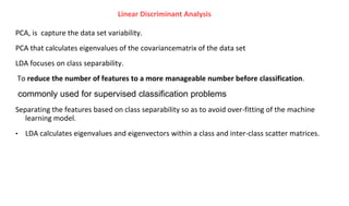
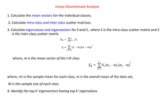
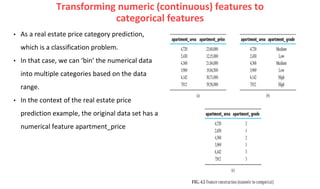
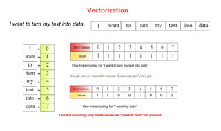
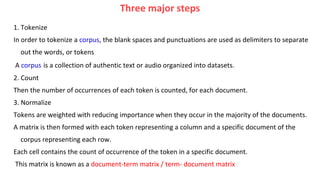
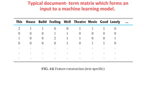
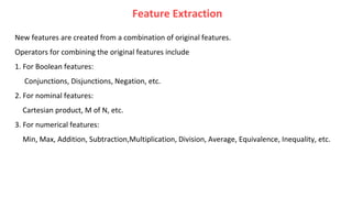
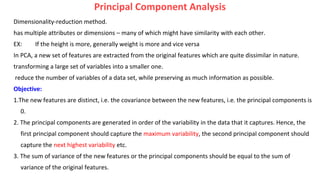
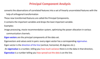
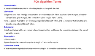
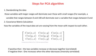
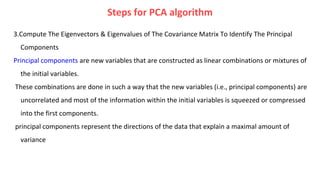
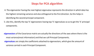
Machine Learning : Feature Engineering
Dr.M.Pyingkodi
Dept of MCA
Kongu Engineering College
Erode, Tamilnadu, India
Basics of Feature Engineering(FE)
• the process of translating a data set into features such that these features are able to represent
the data set more effectively and result in a better learning performance.
• refers to manipulation — addition, deletion, combination, mutation — of your data set to improve
machine learning model training, leading to better performance and greater accuracy.
• a part of the preparatory activities
• It is responsible for taking raw input data and converting that to well-aligned features which are
ready to be used by the machine learning models.
• FE encapsulates various data engineering techniques such as selecting relevant features, handling
missing data, encoding the data, and normalizing it.
• It has two major elements
❖ feature transformation
❖ feature subset selection
Feature
• A feature is an attribute of a data set that is used in a machine learning process.
• selection of the subset of features which are meaningful for machine learning is a sub-area of
feature engineering.
• The features in a data set are also called its dimensions.
• a data set having ‘n’ features is called an n-dimensional data set.
Class variable
- Species
predictor variables
5 dimensional dataset
Feature transformation
Apply a mathematical formula to a particular column(feature) and transform the values which are
useful for our further analysis.
Creating new features from existing features that may help in improving the model performance.
A set of features (m) to create a new feature set (n) while retaining as much information as possible
It has two major elements:
1. feature construction
2. feature extraction
Both are sometimes known as feature discovery
There are two distinct goals of feature transformation:
1. Achieving best reconstruction of the original features in the data set
2. Achieving highest efficiency in the learning task
Feature Construction
Involves transforming a given set of input features to generate a new set of more powerful features.
The data set has three features –
apartment length,
apartment breadth, and
price of the apartment.
If it is used as an input to a regression problem, such data can be training data for the regression model.
So given the training data, the model should be able to predict the price of an apartment whose price is not
known or which has just come up for sale.
However, instead of using length and breadth of the apartment as a predictor, it is much convenient and
makes more sense to use the area of the apartment, which is not an existing feature of the data set.
So such a feature, namely apartment area, can be added to the data set.
In other words, we transform the three- dimensional data set to a four-dimensional data set,
with the newly ‘discovered’ feature apartment area being added to the original data set.
Feature Construction
• when features have categorical value and machine learning needs numeric value inputs
• when features having numeric (continuous) values and need to be converted to ordinal values
• when text-specific feature construction needs to be done
Ordinal data are discrete integers that can be ranked or sorted
Encoding categorical (nominal) variables
FIG. 4.3 Feature construction (encoding nominal variables)
Encoding categorical (ordinal) variables
• The grade is an ordinal variable
with values A, B, C, and D.
• To transform this variable to a
numeric variable, we can create
a feature num_grade mapping a
numeric value against each
ordinal value.
• mapped to values 1, 2, 3, and 4
in the transformed variable
Transforming numeric (continuous) features to
categorical features
• As a real estate price category prediction,
which is a classification problem.
• In that case, we can ‘bin’ the numerical data
into multiple categories based on the data
range.
• In the context of the real estate price
prediction example, the original data set has a
numerical feature apartment_price
Text-specific feature construction
Text is arguably the most predominant medium of communication.
Text mining is an important area of research
unstructured nature of the data
All machine learning models need numerical data as input.
So the text data in the data sets need to be transformed into numerical features
EX:
Facebook or micro-blogging channels like Twitter or emails or short messaging services such as
Whatsapp, Text plays a major role in the flow of information.
Vectorization:
Turning text into vectors/ arrays
To turn text to integer (or boolean, or floating numbers) vectors.
vectors are lists with n positions.
Vectorization
I want to turn my text into data.
One-hot encoding for “I want to turn my text into data”
One-hot encoding for “I want my data”.
One hot encoding only treats values as “present” and “not present”.
Three major steps
1. Tokenize
In order to tokenize a corpus, the blank spaces and punctuations are used as delimiters to separate
out the words, or tokens
A corpus is a collection of authentic text or audio organized into datasets.
2. Count
Then the number of occurrences of each token is counted, for each document.
3. Normalize
Tokens are weighted with reducing importance when they occur in the majority of the documents.
A matrix is then formed with each token representing a column and a specific document of the
corpus representing each row.
Each cell contains the count of occurrence of the token in a specific document.
This matrix is known as a document-term matrix / term- document matrix
Typical document- term matrix which forms an
input to a machine learning model.
Feature Extraction
New features are created from a combination of original features.
Operators for combining the original features include
1. For Boolean features:
Conjunctions, Disjunctions, Negation, etc.
2. For nominal features:
Cartesian product, M of N, etc.
3. For numerical features:
Min, Max, Addition, Subtraction,Multiplication, Division, Average, Equivalence, Inequality, etc.
Feature Extraction
Principal Component Analysis
Dimensionality-reduction method.
has multiple attributes or dimensions – many of which might have similarity with each other.
EX: If the height is more, generally weight is more and vice versa
In PCA, a new set of features are extracted from the original features which are quite dissimilar in nature.
transforming a large set of variables into a smaller one.
reduce the number of variables of a data set, while preserving as much information as possible.
Objective:
1.The new features are distinct, i.e. the covariance between the new features, i.e. the principal components is
0.
2. The principal components are generated in order of the variability in the data that it captures. Hence, the
first principal component should capture the maximum variability, the second principal component should
capture the next highest variability etc.
3. The sum of variance of the new features or the principal components should be equal to the sum of
variance of the original features.
Principal Component Analysis
converts the observations of correlated features into a set of linearly uncorrelated features with the
help of orthogonal transformation
These new transformed features are called the Principal Components.
it contains the important variables and drops the least important variable.
Examples:
image processing, movie recommendation system, optimizing the power allocation in various
communication channels.
Eigen vectors are the principal components of the data set.
Eigenvectors and values exist in pairs: every eigen vector has a corresponding eigenvalue.
Eigen vector is the direction of the line (vertical, horizontal, 45 degrees etc.).
An eigenvalue is a number, telling you how much variance there is in the data in that direction,
Eigenvalue is a number telling you how spread out the data is on the line.
PCA algorithm Terms
Dimensionality
It is the number of features or variables present in the given dataset.
Correlation
It signifies that how strongly two variables are related to each other. Such as if one changes, the other
variable also gets changed. The correlation value ranges from -1 to +1.
Here, -1 occurs if variables are inversely proportional to each other, and +1 indicates that variables are
directly proportional to each other.
Orthogonal
It defines that variables are not correlated to each other, and hence the correlation between the pair of
variables is zero.
Eigenvectors
column vector.
Eigenvalue can be referred to as the strength of the transformation
Covariance Matrix
A matrix containing the covariance between the pair of variables is called the Covariance Matrix.
Steps for PCA algorithm
1. Standardizing the data
those variables with larger ranges will dominate over those with small ranges (For example, a
variable that ranges between 0 and 100 will dominate over a variable that ranges between 0 and
2. Covariance Matrix Calculation
how the variables of the input data set are varying from the mean with respect to each other.
if positive then : the two variables increase or decrease together (correlated)
if negative then : One increases when the other decreases (Inversely correlated)
Steps for PCA algorithm
3.Compute The Eigenvectors & Eigenvalues of The Covariance Matrix To Identify The Principal
Components
Principal components are new variables that are constructed as linear combinations or mixtures of
the initial variables.
These combinations are done in such a way that the new variables (i.e., principal components) are
uncorrelated and most of the information within the initial variables is squeezed or compressed
into the first components.
principal components represent the directions of the data that explain a maximal amount of
variance
4. The eigenvector having the next highest eigenvalue represents the direction in which data has
the highest remaining variance and also orthogonal to the first direction. So this helps in
identifying the second principal component.
5. Like this, identify the top ‘k’ eigenvectors having top ‘k’ eigenvalues so as to get the ‘k’ principal
components.
eigenvectors of the Covariance matrix are actually the directions of the axes where there is the
most variance(most information) and that we call Principal Components.
eigenvalues are simply the coefficients attached to eigenvectors, which give the amount of
variance carried in each Principal Component.
Steps for PCA algorithm
• a matrix is a factorization of that matrix into three matrices.
• linear transformations
SVD of a matrix A (m × n) is a factorization of the form:
• two orthogonal matrices U and V and diagonal matrix D.
• where, U and V are orthonormal matrices
• U is an m × m unitary matrix,
• V is an n × n unitary matrix and
• Σ is an m × n rectangular diagonal matrix.
• The diagonal entries of Σ are known as singular values of matrix A.
• The columns of U and V are called the left-singular and right-singular vectors of matrix A
• The square roots of these eigenvalues are called singular values.
Singular Value Decomposition
1. Patterns in the attributes are captured by the right-singular vectors, i.e.the columns of V.
2. Patterns among the instances are captured by the left-singular, i.e. the
columns of U.
3. Larger a singular value, larger is the part of the matrix A that it accounts for and its
associated vectors.
4. New data matrix with k’ attributes is obtained using the equation
D = D × [v , v , … , v ]
Thus, the dimensionality gets reduced to k
SVD of a data matrix : properties
PCA, is capture the data set variability.
PCA that calculates eigenvalues of the covariancematrix of the data set
LDA focuses on class separability.
To reduce the number of features to a more manageable number before classification.
commonly used for supervised classification problems
Separating the features based on class separability so as to avoid over-fitting of the machine
learning model.
• LDA calculates eigenvalues and eigenvectors within a class and inter-class scatter matrices.
Linear Discriminant Analysis
1. Calculate the mean vectors for the individual classes.
2. Calculate intra-class and inter-class scatter matrices.
3. Calculate eigenvalues and eigenvectors for S and S , where S is the intra-class scatter matrix and S
is the inter-class scatter matrix
where, mi is the sample mean for each class, m is the overall mean of the data set,
Ni is the sample size of each class
4. Identify the top k’ eigenvectors having top k’ eigenvalues
Linear Discriminant Analysis
where, m is the mean vector of the i-th class

Feature Engineering in Machine Learning

  • 1.
    Machine Learning :Feature Engineering Dr.M.Pyingkodi Dept of MCA Kongu Engineering College Erode, Tamilnadu, India
  • 2.
    Basics of FeatureEngineering(FE) • the process of translating a data set into features such that these features are able to represent the data set more effectively and result in a better learning performance. • refers to manipulation — addition, deletion, combination, mutation — of your data set to improve machine learning model training, leading to better performance and greater accuracy. • a part of the preparatory activities • It is responsible for taking raw input data and converting that to well-aligned features which are ready to be used by the machine learning models. • FE encapsulates various data engineering techniques such as selecting relevant features, handling missing data, encoding the data, and normalizing it. • It has two major elements ❖ feature transformation ❖ feature subset selection
  • 3.
    Feature • A featureis an attribute of a data set that is used in a machine learning process. • selection of the subset of features which are meaningful for machine learning is a sub-area of feature engineering. • The features in a data set are also called its dimensions. • a data set having ‘n’ features is called an n-dimensional data set. Class variable - Species predictor variables 5 dimensional dataset
  • 4.
    Feature transformation Apply amathematical formula to a particular column(feature) and transform the values which are useful for our further analysis. Creating new features from existing features that may help in improving the model performance. A set of features (m) to create a new feature set (n) while retaining as much information as possible It has two major elements: 1. feature construction 2. feature extraction Both are sometimes known as feature discovery There are two distinct goals of feature transformation: 1. Achieving best reconstruction of the original features in the data set 2. Achieving highest efficiency in the learning task
  • 5.
    Feature Construction Involves transforminga given set of input features to generate a new set of more powerful features. The data set has three features – apartment length, apartment breadth, and price of the apartment. If it is used as an input to a regression problem, such data can be training data for the regression model. So given the training data, the model should be able to predict the price of an apartment whose price is not known or which has just come up for sale. However, instead of using length and breadth of the apartment as a predictor, it is much convenient and makes more sense to use the area of the apartment, which is not an existing feature of the data set. So such a feature, namely apartment area, can be added to the data set. In other words, we transform the three- dimensional data set to a four-dimensional data set, with the newly ‘discovered’ feature apartment area being added to the original data set.
  • 6.
    Feature Construction • whenfeatures have categorical value and machine learning needs numeric value inputs • when features having numeric (continuous) values and need to be converted to ordinal values • when text-specific feature construction needs to be done Ordinal data are discrete integers that can be ranked or sorted
  • 7.
    Encoding categorical (nominal)variables FIG. 4.3 Feature construction (encoding nominal variables)
  • 8.
    Encoding categorical (ordinal)variables • The grade is an ordinal variable with values A, B, C, and D. • To transform this variable to a numeric variable, we can create a feature num_grade mapping a numeric value against each ordinal value. • mapped to values 1, 2, 3, and 4 in the transformed variable
  • 9.
    Transforming numeric (continuous)features to categorical features • As a real estate price category prediction, which is a classification problem. • In that case, we can ‘bin’ the numerical data into multiple categories based on the data range. • In the context of the real estate price prediction example, the original data set has a numerical feature apartment_price
  • 10.
    Text-specific feature construction Textis arguably the most predominant medium of communication. Text mining is an important area of research unstructured nature of the data All machine learning models need numerical data as input. So the text data in the data sets need to be transformed into numerical features EX: Facebook or micro-blogging channels like Twitter or emails or short messaging services such as Whatsapp, Text plays a major role in the flow of information. Vectorization: Turning text into vectors/ arrays To turn text to integer (or boolean, or floating numbers) vectors. vectors are lists with n positions.
  • 11.
    Vectorization I want toturn my text into data. One-hot encoding for “I want to turn my text into data” One-hot encoding for “I want my data”. One hot encoding only treats values as “present” and “not present”.
  • 12.
    Three major steps 1.Tokenize In order to tokenize a corpus, the blank spaces and punctuations are used as delimiters to separate out the words, or tokens A corpus is a collection of authentic text or audio organized into datasets. 2. Count Then the number of occurrences of each token is counted, for each document. 3. Normalize Tokens are weighted with reducing importance when they occur in the majority of the documents. A matrix is then formed with each token representing a column and a specific document of the corpus representing each row. Each cell contains the count of occurrence of the token in a specific document. This matrix is known as a document-term matrix / term- document matrix
  • 13.
    Typical document- termmatrix which forms an input to a machine learning model.
  • 14.
    Feature Extraction New featuresare created from a combination of original features. Operators for combining the original features include 1. For Boolean features: Conjunctions, Disjunctions, Negation, etc. 2. For nominal features: Cartesian product, M of N, etc. 3. For numerical features: Min, Max, Addition, Subtraction,Multiplication, Division, Average, Equivalence, Inequality, etc.
  • 15.
  • 16.
    Principal Component Analysis Dimensionality-reductionmethod. has multiple attributes or dimensions – many of which might have similarity with each other. EX: If the height is more, generally weight is more and vice versa In PCA, a new set of features are extracted from the original features which are quite dissimilar in nature. transforming a large set of variables into a smaller one. reduce the number of variables of a data set, while preserving as much information as possible. Objective: 1.The new features are distinct, i.e. the covariance between the new features, i.e. the principal components is 0. 2. The principal components are generated in order of the variability in the data that it captures. Hence, the first principal component should capture the maximum variability, the second principal component should capture the next highest variability etc. 3. The sum of variance of the new features or the principal components should be equal to the sum of variance of the original features.
  • 17.
    Principal Component Analysis convertsthe observations of correlated features into a set of linearly uncorrelated features with the help of orthogonal transformation These new transformed features are called the Principal Components. it contains the important variables and drops the least important variable. Examples: image processing, movie recommendation system, optimizing the power allocation in various communication channels. Eigen vectors are the principal components of the data set. Eigenvectors and values exist in pairs: every eigen vector has a corresponding eigenvalue. Eigen vector is the direction of the line (vertical, horizontal, 45 degrees etc.). An eigenvalue is a number, telling you how much variance there is in the data in that direction, Eigenvalue is a number telling you how spread out the data is on the line.
  • 18.
    PCA algorithm Terms Dimensionality Itis the number of features or variables present in the given dataset. Correlation It signifies that how strongly two variables are related to each other. Such as if one changes, the other variable also gets changed. The correlation value ranges from -1 to +1. Here, -1 occurs if variables are inversely proportional to each other, and +1 indicates that variables are directly proportional to each other. Orthogonal It defines that variables are not correlated to each other, and hence the correlation between the pair of variables is zero. Eigenvectors column vector. Eigenvalue can be referred to as the strength of the transformation Covariance Matrix A matrix containing the covariance between the pair of variables is called the Covariance Matrix.
  • 19.
    Steps for PCAalgorithm 1. Standardizing the data those variables with larger ranges will dominate over those with small ranges (For example, a variable that ranges between 0 and 100 will dominate over a variable that ranges between 0 and 2. Covariance Matrix Calculation how the variables of the input data set are varying from the mean with respect to each other. if positive then : the two variables increase or decrease together (correlated) if negative then : One increases when the other decreases (Inversely correlated)
  • 20.
    Steps for PCAalgorithm 3.Compute The Eigenvectors & Eigenvalues of The Covariance Matrix To Identify The Principal Components Principal components are new variables that are constructed as linear combinations or mixtures of the initial variables. These combinations are done in such a way that the new variables (i.e., principal components) are uncorrelated and most of the information within the initial variables is squeezed or compressed into the first components. principal components represent the directions of the data that explain a maximal amount of variance
  • 21.
    4. The eigenvectorhaving the next highest eigenvalue represents the direction in which data has the highest remaining variance and also orthogonal to the first direction. So this helps in identifying the second principal component. 5. Like this, identify the top ‘k’ eigenvectors having top ‘k’ eigenvalues so as to get the ‘k’ principal components. eigenvectors of the Covariance matrix are actually the directions of the axes where there is the most variance(most information) and that we call Principal Components. eigenvalues are simply the coefficients attached to eigenvectors, which give the amount of variance carried in each Principal Component. Steps for PCA algorithm
  • 22.
    • a matrixis a factorization of that matrix into three matrices. • linear transformations SVD of a matrix A (m × n) is a factorization of the form: • two orthogonal matrices U and V and diagonal matrix D. • where, U and V are orthonormal matrices • U is an m × m unitary matrix, • V is an n × n unitary matrix and • Σ is an m × n rectangular diagonal matrix. • The diagonal entries of Σ are known as singular values of matrix A. • The columns of U and V are called the left-singular and right-singular vectors of matrix A • The square roots of these eigenvalues are called singular values. Singular Value Decomposition
  • 23.
    1. Patterns inthe attributes are captured by the right-singular vectors, i.e.the columns of V. 2. Patterns among the instances are captured by the left-singular, i.e. the columns of U. 3. Larger a singular value, larger is the part of the matrix A that it accounts for and its associated vectors. 4. New data matrix with k’ attributes is obtained using the equation D = D × [v , v , … , v ] Thus, the dimensionality gets reduced to k SVD of a data matrix : properties
  • 24.
    PCA, is capturethe data set variability. PCA that calculates eigenvalues of the covariancematrix of the data set LDA focuses on class separability. To reduce the number of features to a more manageable number before classification. commonly used for supervised classification problems Separating the features based on class separability so as to avoid over-fitting of the machine learning model. • LDA calculates eigenvalues and eigenvectors within a class and inter-class scatter matrices. Linear Discriminant Analysis
  • 25.
    1. Calculate themean vectors for the individual classes. 2. Calculate intra-class and inter-class scatter matrices. 3. Calculate eigenvalues and eigenvectors for S and S , where S is the intra-class scatter matrix and S is the inter-class scatter matrix where, mi is the sample mean for each class, m is the overall mean of the data set, Ni is the sample size of each class 4. Identify the top k’ eigenvectors having top k’ eigenvalues Linear Discriminant Analysis where, m is the mean vector of the i-th class