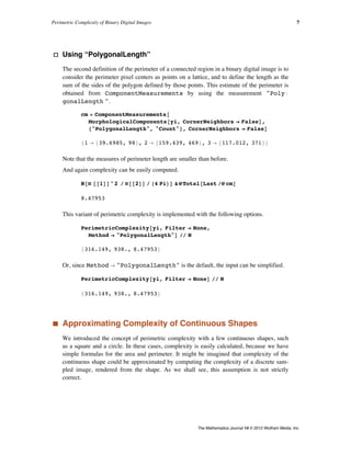
This document discusses the concept of perimetric complexity, a measure of the complexity of binary digital images defined as the sum of inside and outside perimeters of the foreground, squared, divided by the foreground area. It explores the challenges of applying this measure to digital images and proposes a new metric called visual perimetric complexity, which accounts for the human visual system's limitations. Additionally, the article provides Mathematica functions for calculating perimetric complexity and presents examples of its application in image processing.
![The Mathematica®
Journal
Perimetric Complexity of
Binary Digital Images
Notes on Calculation and Relation to Visual
Complexity
Andrew B. Watson
Perimetric complexity is a measure of the complexity of binary
pictures. It is defined as the sum of inside and outside
perimeters of the foreground, squared, divided by the foreground
area, divided by 4 p. Difficulties arise when this definition is
applied to digital images composed of binary pixels. In this
article we identify these problems and propose solutions.
Perimetric complexity is often used as a measure of visual
complexity, in which case it should take into account the limited
resolution of the visual system. We propose a measure of visual
perimetric complexity that meets this requirement.
‡ Background
Perimetric complexity is a measure of the complexity of binary pictures. It is defined as
the sum of inside and outside perimeters of the foreground, squared, divided by the fore-
ground area, divided by 4 p. The concept of perimetric complexity was first introduced
(and called dispersion) by Attneave and Arnoult [1] in an effort to explain the apparent per-
ceptual complexity of visual shapes. In the field of image processing, the concept appears
as its inverse, compactness [2, 3, 4]. The concept was given new life (and a new name) in
2006 by Pelli et al., who showed that the efficiency of letter identification was nearly pro-
portional to perimetric complexity [5]. It has since become a popular metric in a variety of
shape analysis applications, including human letter identification [5, 6, 7], handwriting
recognition [8], evolution of graphical symbols [9], and design of graphical anti-spam tech-
nologies [10, 11, 12].
In this article we develop Mathematica functions to compute perimetric complexity of bi-
nary digital images and illustrate their application. The code is compatible with Version 8
of Mathematica.
The Mathematica Journal 14 © 2012 Wolfram Media, Inc.](https://image.slidesharecdn.com/watson-210224032444/85/Perimetric-Complexity-of-Binary-Digital-Images-1-320.jpg)
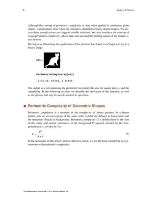
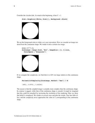
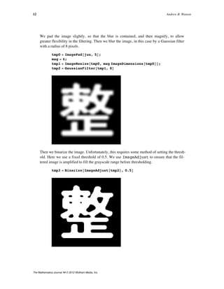
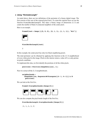
![We begin with the example of a circular disk with unit radius.
Graphics@8White, Disk@D<, PlotRange Ø 2, Background Ø BlackD
Here the perimeter is 2 p and the area is p, so the complexity is
(2)
C =
H2 pL2
4 p p
= 1.
It can be shown that the disk is the shape with the lowest complexity. The normalizing con-
stant 4 p in the definition leads to a unit value for this most simple shape. As a conse-
quence, any other value of complexity is easily compared to that of the circular disk. Pelli
et al. [5] suggest that complexity is closely related to the number of visual features in a
shape. In that sense, we could say that the circular disk has only a single feature.
Our next example is a square with unit sides.
The perimeter here is 4, and the area is 1, so the perimetric complexity is
(3)
C =
42
4 p
=
4
p
º 1.27.
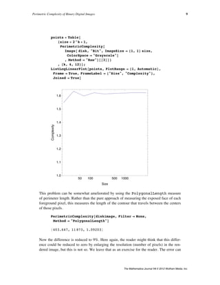
If we add a square hole in the center with side length 1/2, there is an interior perimeter as
well, as shown here.
Graphics@8
White, Rectangle@-81, 1< ê 2, 81, 1< ê 2D,
Black, Rectangle@-81, 1< ê 4, 81, 1< ê 4D<,
PlotRange Ø 1, Background Ø BlackD
Now the total perimeter is the sum of inner and outer perimeters and the area is the differ-
ence in areas of the squares, so
Perimetric Complexity of Binary Digital Images 3
The Mathematica Journal 14 © 2012 Wolfram Media, Inc.](https://image.slidesharecdn.com/watson-210224032444/85/Perimetric-Complexity-of-Binary-Digital-Images-3-320.jpg)
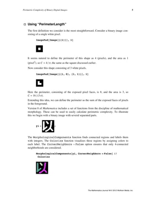
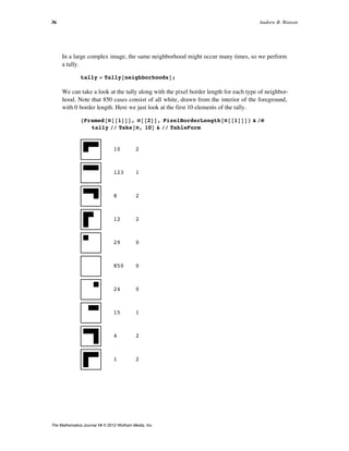
![Now the total perimeter is the sum of inner and outer perimeters and the area is the differ-
ence in areas of the squares, so
(4)
C =
H4 + 2L2
H1 - 1 ê 4L 4 p
=
12
p
º 3.82.
So according to this measure, the square with a hole is about three times as complex as the
square.
Some important observations about complexity are: (1) it is dimensionless; (2) it is inde-
pendent of scale or orientation; and (3) it is additive. By additive we mean that the
complexity of a pair of shapes, considered as a single shape, is equal to the sum of their
complexities computed separately.
‡ Perimetric Complexity of Plane Curves
Although it is beyond the scope of this article, we note for reference that if a shape is de-
fined by a closed parametric curve, its exact complexity can be obtained using calculus
methods [13]. Specifically, if over an interval a § t § b the functions xHtL and yHtL and
their derivatives x
°
HtL and y
°
HtL are continuous, then the curve described has a length
(5)
P = ‡
a
b
x
° 2
+ y
° 2
dt
and an area
(6)
A = -‡
a
b
y
°
x dt.
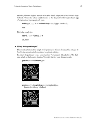
‡ Perimetric Complexity of Binary Digital Images
A digital image is defined here as a rectangular array of square pixels. A binary digital im-
age contains pixel values of 1 (white) and 0 (black) only. The foreground consists of the
white pixels.
The original definition of complexity relies upon the notion of a perimeter, which has no
unique analog in the context of digital images. However, two definitions of perimeter are
available, as described below.
4 Andrew B. Watson
The Mathematica Journal 14 © 2012 Wolfram Media, Inc.](https://image.slidesharecdn.com/watson-210224032444/85/Perimetric-Complexity-of-Binary-Digital-Images-4-320.jpg)
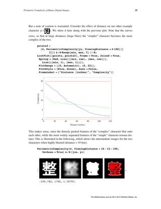
![Now the difference is reduced to 9%. Here again, the reader might think that this differ-
ence could be reduced to zero by enlarging the resolution (number of pixels) in the ren-
never be zero, because the path between pixel centers must always be vertical, horizontal,
or diagonal, so it can never smoothly follow the true circular contour. Put another way, it
has a higher fractal dimension than the circle, and thus greater length.
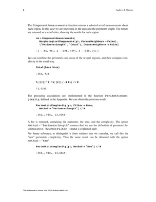
‡ Pelli Algorithm
Pelli et al. [2] proposed a method for computing complexity that we quote here in full:
The ink area is the number of 1’s. To measure the perimeter we first replace the
image by its outline. (We OR the image with translations of the original, shifted
by one pixel left; left and up; up; up and right; right; right and down; down; and
down and left; and then bit clear with the original image. This leaves a one-
pixel-thick outline.) It might seem enough to just count the 1’s in this outline im-
age, but the resulting “lengths” are not Euclidean: diagonal lines have “lengths”
equal to that of their base plus height. Instead we first thicken the outline. (We
OR the outline image with translations of the original outline, shifted by one
pixel left; up; right; and down.) This leaves a three-pixel-thick outline. We then
count the number of 1’s and divide by 3.
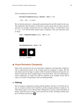
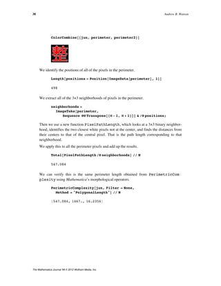
This method can be implemented using the Dilation function, as we show here. With
verbose ã True, it shows two images: the perimeter in red and the thickened perime-
ter. It returns the length of the perimeter, the area, and the complexity.
PelliMethod@image_, verbose_: FalseD := Module@
8tmp0, tmp1, tmp2, tmp3, perimeter, area, result<,
tmp0 = ImagePad@image, 2D;
tmp1 = Dilation@tmp0, BoxMatrix@1DD;
tmp2 = ImageSubtract@tmp1, tmp0D;
tmp3 = Dilation@tmp2, CrossMatrix@1DD;
perimeter = Total@ImageData@tmp3D, 2D ê 3;
area = Total@ImageData@tmp0D, 2D;
result = 8perimeter, area, perimeter^2 ê area ê H4 PiL<;
If@verbose, Column@8GraphicsRow@
8ColorCombine@8tmp1, tmp0, tmp0<D, tmp3<D, result<D,
resultD
D
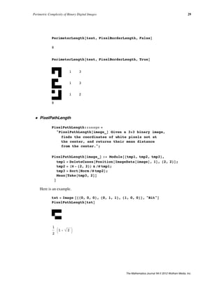
We apply this to the three-component Chinese character.
PelliMethod@yi, TrueD êê N
8326.333, 938., 9.03463<
10 Andrew B. Watson
The Mathematica Journal 14 © 2012 Wolfram Media, Inc.](https://image.slidesharecdn.com/watson-210224032444/85/Perimetric-Complexity-of-Binary-Digital-Images-10-320.jpg)
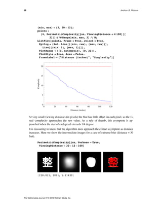
![And because we imagine that the image is viewed at such a distance that the pixels are not
resolved, we use the (default) PolygonalLength method.
PerimetricComplexity@tmp3, Filter Ø NoneD
81944.82, 24 044, 12.5182<
We can compare this to the unfiltered raw complexity.
PerimetricComplexity@jun, Method Ø "Raw"D êê N
8606., 1467., 19.9207<
The filtered version has substantially lower complexity, as we expect.
· Visual Filtering Using a Gaussian
For the filtering to approximate visual blur, it must be based on the size of the original im-
age and its distance from the viewer. Obviously, as the shape becomes smaller or farther
from the observer, its details are more blurred, less visible, and contribute less to the vi-
sual complexity.
The challenge is to determine the appropriate value of the Gaussian filter radius for a
given viewing distance. From measurements of visual sensitivity, we know that visual
Gaussian blur has a standard deviation of about B = 0.01549 degrees of visual angle [11].
But we need to convert this into a radius in pixels. Recall that the image may be magni-
fied by M before filtering. If we express the viewing distance V in terms of pixels (before
magnification), then the size of each pixel S (after magnification) is approximately
(7)
S =
57.3
MV
deg.
The constant 57.3 is an approximation to 1 ê arctanH1°L.
1. ê ArcTan@1 °D
57.3016
By default, the radius is twice the standard deviation. So the filter radius should be
(8)
R =
2 B
S
=
2 BMV
57.3
pixel.
Perimetric Complexity of Binary Digital Images 13
The Mathematica Journal 14 © 2012 Wolfram Media, Inc.](https://image.slidesharecdn.com/watson-210224032444/85/Perimetric-Complexity-of-Binary-Digital-Images-13-320.jpg)
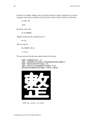
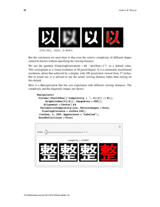
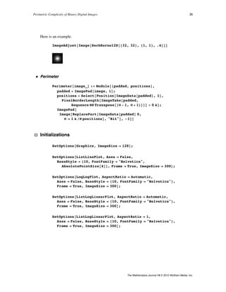
![The preceding steps of padding, magnification, and filtering are built into the function
PerimetricComplexity, as shown below. With Verbose Ø True, the function
also shows the original, the filtered version, the binarized version, and the original (in red)
with the perimeter of the filtered version (in white within the original and aqua outside the
original).
PerimetricComplexity@jun, Magnification Ø 4,
Filter Ø "Gaussian", ViewingDistance -> 48 µ 72,
Verbose Ø TrueD
81987.85, 23 932, 13.1395<
The Gaussian is parameterized by a scale in degrees of visual angle. The default value is
2.33/60 degrees. The user can experiment with different values via the option
GaussianScale.
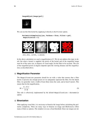
· Accurate Visual Filtering with Sech
Visual blur is more accurately represented with filters other than a Gaussian. In one
simple form, the kernel is a sech (hyperbolic secant) function [14, 15]. This filter can be
selected with an option (Filter Ø "Sech", the default) in the function PerimeÖ
tricComplexity.
PerimetricComplexity@junD
81016.14, 5977, 13.7472<
The hyperbolic secant is parameterized by a scale in degrees of visual angle. The default
value is 2.16/60 degrees [14, 15]. The user can experiment with different values via the op-
tion SechScale.
· Accurate Visual Filtering with an Arbitrary Point Spread Function
In real human eyes, blur results not only from low-order aberrations such as defocus and
astigmatism, but also from higher-order aberrations. In this example, we use a blur
function defined by an array of values representing the filter kernel. This example is an
actual estimate of the point spread function for an individual human observer, as mea-
sured using a device called a wavefront aberrometer that includes both low-order and high-
order aberrations [16].
Perimetric Complexity of Binary Digital Images 15
The Mathematica Journal 14 © 2012 Wolfram Media, Inc.](https://image.slidesharecdn.com/watson-210224032444/85/Perimetric-Complexity-of-Binary-Digital-Images-15-320.jpg)
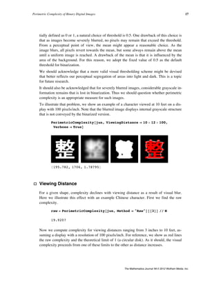
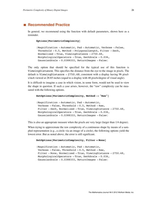
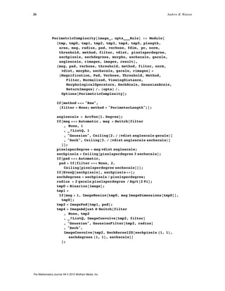
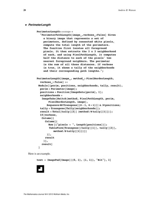
![‡ Examples
We conclude with two examples of the application of PerimetricComplexity.
The first example is a set of three binary images. Below each image we print the
complexity.
pictures = 8cat, horse, family<;
Grid@
8pictures,
TextüStyle@NumberForm@Last@NüPerimetricComplexity@ÒDD,
3D, 14D & êü pictures<
, ItemSize Ø 10, Spacings Ø 2D
3.95 8.62 22.1
The second example is an array of characters. This array was created as part of an experi-
ment on the effect of complexity on visual acuity [6]. The first row is the Sloan letters, a
well-known set of letter acuity targets [5]. The remaining six rows are sets of Chinese char-
acters selected so as to be of equal complexity within a row, but increasing in complexity
from row to row [6]. The metric of complexity used for selection was different from that
developed in this article.
GraphicsGrid@chararrayD
22 Andrew B. Watson
The Mathematica Journal 14 © 2012 Wolfram Media, Inc.](https://image.slidesharecdn.com/watson-210224032444/85/Perimetric-Complexity-of-Binary-Digital-Images-22-320.jpg)


![‡ Acknowledgments
I thank and blame Denis Pelli for introducing me to perimetric complexity [5]. I thank Dr.
Cong Yu for providing the Chinese character optotypes [6]. I thank Albert Ahumada and
Jeffrey Mulligan for useful discussions. I thank Larry Thibos for providing the wavefront
data [16]. This work was supported by NASA Space Human Factors Engineering WBS
466199.
‡ References
[1] F. Attneave and M. D. Arnoult, “The Quantitative Study of Shape and Pattern Perception,”
Psychological Bulletin, 53(6), 1956 pp. 452–471. psycnet.apa.org/journals/bul/53/6/452.
[2] P. V. Sankar and E. V. Krishnamurthy, “On the Compactness of Subsets of Digital Pictures,”
Computer Graphics and Image Processing, 8(1), 1978 pp. 136–143.
www.sciencedirect.com/science/article/pii/S0146664X78800215.
[3] S. Ullman, “The Visual Analysis of Shape and Form,” The Cognitive Neurosciences (M. S.
Gazzaniga, ed.), Cambridge, MA: MIT Press, 1995 pp. 339–350.
[4] R. Montero and E. Bribiesca, “State of the Art of Compactness and Circularity Measures,” In-
ternational Mathematical Forum, 4(27), 2009 pp. 1305–1335.
www.m-hikari.com/imf-password2009/25-28-2009/index.html.
[5] D. G. Pelli, C. W. Burns, B. Farell, and D. C. Moore-Page, “Feature Detection and Letter Iden-
tification,” Vision Research, 46(28), 2006 pp. 4646–4674.
www.psych.nyu.edu/pelli/pubs/pelli2006letters.pdf.
[6] J.-Y. Zhang, T. Zhang, F. Xue, L. Liu, and C. Yu, “Legibility Variations of Chinese Characters
and Implications for Visual Acuity Measurement in Chinese Reading Population,” Investiga-
tive Ophthalmology & Visual Science, 48(5), 2007 pp. 2383–2390.
www.iovs.org/content/48/5/2383.short.
[7] A. B. Watson and A. J. Ahumada, Jr., “Modeling Acuity for Optotypes Varying in Complexity,”
presentation given at The Association for Research in Vision and Ophthalmology Confer-
ence (ARVO 2010), Ft. Lauderdale, FL. abstracts.iovs.org//cgi/content/abstract/51/5/5174.
[8] A. Rusu and V. Govindaraju, “The Influence of Image Complexity on Handwriting Recogni-
tion,” in Proceediings of the Tenth International Workshop on Frontiers in Handwriting Recog-
nition (IWFHR 2006), La Baule (France). hal.inria.fr/inria-00112666/.
[9] S. Garrod, N. Fay, J. Lee, J. Oberlander, and T. MacLeod, “Foundations of Representation:
Where Might Graphical Symbol Systems Come From?,” Cognitive Science, 31(6), 2007 pp.
961–987. onlinelibrary.wiley.com/doi/10.1080/03640210701703659/abstract.
[10] M. Chew and H. Baird, “BaffleText: A Human Interactive Proof,” in Proceedings of the
IS&T/SPIE Document Recognition and Retrieval Conference X (DRR X), Santa Clara, CA,
2003 pp. 305-316. www.imaging.org/IST/store/epub.cfm?abstrid=22585.
[11] B. Biggio, G. Fumera, I. Pillai, and F. Roli, “Image Spam Filtering Using Visual Information,”
in Proceedings of the 14th International Conference on Image Analysis and Processing
(ICIAP 2007), Modena, Italy pp. 105–110.
ieeexplore.ieee.org/xpl/freeabs_all.jsp?arnumber=4362765.
Perimetric Complexity of Binary Digital Images 39
The Mathematica Journal 14 © 2012 Wolfram Media, Inc.](https://image.slidesharecdn.com/watson-210224032444/85/Perimetric-Complexity-of-Binary-Digital-Images-39-320.jpg)
![[12] G. Fumera, I. Pillai, F. Roli, and B. Biggio, “Image Spam Filtering Using Textual and Visual In-
formation,” in Proceedings of the MIT Spam Conference 2007, Cambridge, MA.
projects.csail.mit.edu/spamconf/SC2007/MIT_Spam_Conf _ 2007_Papers.tar.gz.
[13] R. Courant, Differential and Integral Calculus, Vol. 1, 2nd ed. (E. J. McShane, trans.), Lon-
don: Blackie & Son Limited, 1937.
[14] A. B. Watson and A. J. Ahumada, Jr., “A Standard Model for Foveal Detection of Spatial Con-
trast,” Journal of Vision, 5(9), 2005 pp. 717–740. journalofvision.org/5/9/6.
[15] A. B. Watson and A. J. Ahumada, “Blur Clarified: A Review and Synthesis of Blur Discrimina-
tion,” Journal of Vision, 11(5), 2011. journalofvision.org/11/5/10.
[16] L. N. Thibos, X. Hong, A. Bradley, and X. Cheng, “Statistical Variation of Aberration Struc-
ture and Image Quality in a Normal Population of Healthy Eyes,” Journal of the Optical Soci-
ety of America A: Optics, Image Science, and Vision, 19(12), 2002 pp. 2329–2348.
www.opticsinfobase.org/abstract.cfm?URI=josaa-19-12-2329.
A. B. Watson, “Perimetric Complexity of Binary Digital Images,” The Mathematica Journal, 2012.
dx.doi.org/doi:10.3888/tmj.14-5.
About the Author
Andrew B. Watson is the Senior Scientist for Vision Research at NASA. He is editor-in-
chief of the Journal of Vision (journalofvision.org). He is the author of over 150 scientific
papers and four patents. He is a Fellow of the Optical Society of America, the Association
for Research in Vision and Ophthalmology, and the Society for Information Display.
Andrew B. Watson
MS 262-2
NASA Ames Research Center
Moffett Field, CA 94035
andrew.b.watson@nasa.gov
40 Andrew B. Watson
The Mathematica Journal 14 © 2012 Wolfram Media, Inc.](https://image.slidesharecdn.com/watson-210224032444/85/Perimetric-Complexity-of-Binary-Digital-Images-40-320.jpg)