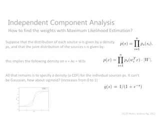
2. INDEPENDENT COMPONENT ANALYSIS
DATA
Imagine that you are a weaver, and you have a loom of colorful strings. Each string
represents a unique pattern in the data. With actual data, each of these strings would be
a vector of numbers that can be fit with a linear equation. As we see the strings above,
they are well organized.
3. MIXED UP DATA
INDEPENDENCE
INDEPENDENT COMPONENT ANALYSIS
Unfortunately, when we collect data in the real world it does not come to us neat and
organized. Our unique strings get mixed up with other strings, and random signal such as
noise. In our example above, a monkey has come along and mixed up our strings. How
do we untangle them?
4. HOW TO UNMIX?
INDEPENDENT COMPONENT ANALYSIS
We could know something special about each string, maybe a feature like color, and manually
unmix, however it we are dealing with a huge dataset and don’t have a clue about any special
features, we are powerless. This is where ICA comes in. We start with our mixed data and
assume 1) we have mixed up data (our loom) that is 2) comprised of independent signals
5. MIXED STRINGS
(OBSERVED DATA)
INDEPENDENT COMPONENT ANALYSIS
=
MONKEY
MADNESS
(“MIXING MATRIX”)
X = A SX
ORIGINAL
STRINGS
(ORIGINAL DATA)
X
We start with this mixed up data, X, and we know that it was generated by the monkey applying
some sequence of movements to it (the “monkey madness”). We call this series of
transformations that the monkey applies to the unmixed data, s our mixing matrix. This matrix
would consist of vectors of numbers that, when multiplied with s, produce the observed data X.
6. INDEPENDENT COMPONENT ANALYSIS
S = A-1 XX
To solve this problem and recover our original strings from the mixed ones, we just need to
solve this equation for s. We know X, so we just need to figure out what the inverse of A is. This
is normally referred to as “W” or the un-mixing matrix. We are going to choose the numbers in
this matrix that maximize the probability of our data.
MIXED STRINGS
(OBSERVED DATA)
=
UN-MIXING
MATRIX, W
ORIGINAL
STRINGS
(ORIGINAL DATA)
X
7. INDEPENDENT COMPONENT ANALYSIS
S = A-1 XX
What is basically done is that we model the CDF of each signal’s probability as the sigmoid
function because it increases from 0 to 1, the derivative of the sigmoid is the density function,
and then we would iteratively maximize that function until convergence to find the weights, this
inverse matrix (details in next slides!)
MIXED STRINGS
(OBSERVED DATA)
=
UN-MIXING
MATRIX, W
ORIGINAL
STRINGS
(ORIGINAL DATA)
X
8. Independent Component Analysis
How to find the weights with Maximum Likelihood Estimation?
Suppose that the distribution of each source si is given by a density
ps, and that the joint distribution of the sources s is given by:
this implies the following density on x = As = W1s
All that remains is to specify a density (a CDF) for the individual sources ps. It can’t
be Gaussian, how about sigmoid? (increases from 0 to 1)
CS229 Notes, Andrew Ng, 2012
9. So we model the CDF for each independent signal with sigmoid, so to get the
probability of the signal at any particular time-point we look at the derivative of the CDF
(the PDF):
So if we want to maximize this probability (find our data), we want to make it as big as
possible. The square matrix W is the parameter in our model, so given a training set,
the log likelihood is given by:
And we want to maximize this in terms of W. It’s useful to know that:
And so a “one at a time” (stochastic gradient ascent rule) is:
This is how we would update our weights until convergence.
Independent Component Analysis
How to find the weights with Maximum Likelihood Estimation?
CS229 Notes, Andrew Ng, 2012
10. FastICA Modification
“ICA with Reference” is a modification of FastICA
CS229 Notes, Andrew Ng, 2012
Negative entropy is used to measure mutual independence in formula:
1st term: Gaussian variable (wTx), 2nd non-quadratic contrast function
||w||2 = 1 used when maximizing J(y) such that:
If we choose, for the 2nd function G’’’(u) = u3, the update becomes:
“Inspired” by this form of the update, we can impose an additional
constraint that incorporates prior information about the components
so it no longer maximizes just independence, but is also close to the
reference, r:
11. ICA CAVEATS
Permutation of the original sources is ambiguous
But this doesn’t matter for most applications
Data assumed to be non-Gaussian
If the data is Gaussian, there is an arbitrary rotational component in the
mixing matrix that cannot be determined from the data, so we cannot
recover the original sources
No way to recover scaling of the weights
If a single column of matrix A were scaled by a factor of 2 and the
corresponding source were scaled by a factor of ½, then there is again no
way, given only the x(i)’s, to determine this had happened.
12. Why can’t the data be Gaussian?
“Suppose we observe some x = As, where A is our mixing matrix. The distribution of x
will also be Gaussian, with zero mean and covariance
E[xxT ] = E[AssTAT ] = AAT
Now, let R be an arbitrary orthogonal (less formally, a rotation/reflection) matrix, so
that RRT = RTR = I, and let A’ = AR. Then if the data had been mixed according to A’
instead of A, we would have instead observed x’ = A’s. The distribution of x’ is
also Gaussian, with zero mean and covariance
E[x’(x’)T ] = E[A’ssT (A’)T ] = E[ARssT (AR)T ] = ARRTAT = AAT
Hence, whether the mixing matrix is A or A’, we would observe data from a N(0;AAT )
distribution. Thus, there is no way to tell if the sources were mixed using A and A’. So,
there is an arbitrary rotational component in the mixing matrix that cannot be
determined from the data, and we cannot recover the original sources.”
CS229 Notes, Andrew Ng, 2012