polymer

1. Principal component Analysis
(Feature Selection Techniques)

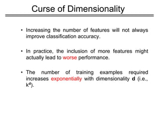
2. Curse of Dimensionality
• Increasing the number of features will not always
improve classification accuracy.
• In practice, the inclusion of more features might
actually lead to worse performance.
• The number of training examples required
increases exponentially with dimensionality d (i.e.,
kd
).

3. 3
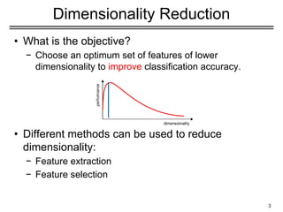
Dimensionality Reduction
• What is the objective?
− Choose an optimum set of features of lower
dimensionality to improve classification accuracy.
• Different methods can be used to reduce
dimensionality:
− Feature extraction
− Feature selection

4. 4
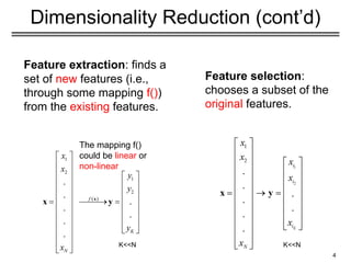
Dimensionality Reduction (cont’d)
Feature extraction: finds a
set of new features (i.e.,
through some mapping f())
from the existing features.
Feature selection:
chooses a subset of the
original features.
The mapping f()
could be linear or
non-linear
K<<N K<<N

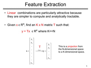
5. Feature Extraction
• Linear combinations are particularly attractive because
they are simpler to compute and analytically tractable.
• Given x ϵ RN
, find an K x N matrix T such that:
y = Tx ϵ RK
where K<<N
5
T This is a projection from
the N-dimensional space
to a K-dimensional space.

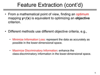
6. Feature Extraction (cont’d)
• From a mathematical point of view, finding an optimum
mapping y=𝑓(x) is equivalent to optimizing an objective
criterion.
• Different methods use different objective criteria, e.g.,
− Minimize Information Loss: represent the data as accurately as
possible in the lower-dimensional space.
− Maximize Discriminatory Information: enhance the
class-discriminatory information in the lower-dimensional space.
6

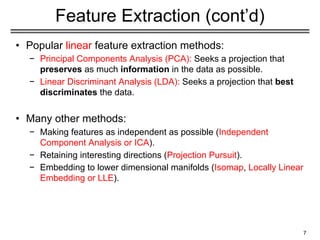
7. Feature Extraction (cont’d)
• Popular linear feature extraction methods:
− Principal Components Analysis (PCA): Seeks a projection that
preserves as much information in the data as possible.
− Linear Discriminant Analysis (LDA): Seeks a projection that best
discriminates the data.
• Many other methods:
− Making features as independent as possible (Independent
Component Analysis or ICA).
− Retaining interesting directions (Projection Pursuit).
− Embedding to lower dimensional manifolds (Isomap, Locally Linear
Embedding or LLE).
7

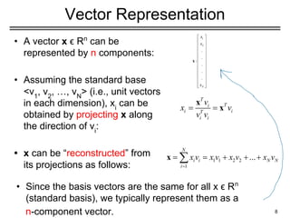
8. Vector Representation
• A vector x ϵ Rn
can be
represented by n components:
• Assuming the standard base
<v1
, v2
, …, vN
> (i.e., unit vectors
in each dimension), xi
can be
obtained by projecting x along
the direction of vi
:
• x can be “reconstructed” from
its projections as follows:
8
• Since the basis vectors are the same for all x ϵ Rn
(standard basis), we typically represent them as a
n-component vector.

9. Vector Representation (cont’d)
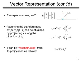
• Example assuming n=2:
• Assuming the standard base
<v1
=i, v2
=j>, xi
can be obtained
by projecting x along the
direction of vi
:
• x can be “reconstructed” from
its projections as follows:
9
i
j

10. 10
Principal Component Analysis (PCA)
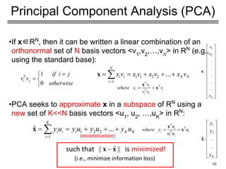
•If x∈RN
, then it can be written a linear combination of an
orthonormal set of N basis vectors <v1
,v2
,…,v𝑁
> in RN
(e.g.,
using the standard base):
•PCA seeks to approximate x in a subspace of RN
using a
new set of K<<N basis vectors <u1
, u2
, …,uK
> in RN
:
such that is minimized!
(i.e., minimize information loss)
(reconstruction)

11. 11
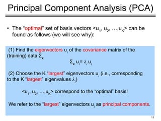
Principal Component Analysis (PCA)
• The “optimal” set of basis vectors <u1
, u2
, …,uK
> can be
found as follows (we will see why):
(1) Find the eigenvectors u𝑖
of the covariance matrix of the
(training) data Σx
Σx
u𝑖
= 𝜆𝑖
u𝑖
(2) Choose the K “largest” eigenvectors u𝑖
(i.e., corresponding
to the K “largest” eigenvalues 𝜆𝑖
)
<u1
, u2
, …,uK
> correspond to the “optimal” basis!
We refer to the “largest” eigenvectors u𝑖
as principal components.

12. • Suppose we are given x1
, x2
, ..., xM
(N x 1) vectors
Step 1: compute sample mean
Step 2: subtract sample mean (i.e., center data at zero)
Step 3: compute the sample covariance matrix Σx
12
PCA - Steps
N: # of features
M: # data
where A=[Φ1
Φ2
... ΦΜ
]
i.e., the columns of A are the Φi
(N x M matrix)

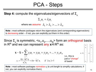
13. Step 4: compute the eigenvalues/eigenvectors of Σx
Since Σx
is symmetric, <u1
,u2
,…,uN
> form an orthogonal basis
in RN
and we can represent any x∈RN
as:
13
PCA - Steps
Note : most software packages return the eigenvalues (and corresponding eigenvectors)
is decreasing order – if not, you can explicitly put them in this order)
where we assume
Note : most software packages normalize ui
to unit length to simplify calculations; if
not, you can explicitly normalize them)
i.e., this is
just a “change”
of basis!

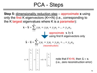
14. Step 5: dimensionality reduction step – approximate x using
only the first K eigenvectors (K<<N) (i.e., corresponding to
the K largest eigenvalues where K is a parameter):
14
PCA - Steps
approximate
using first K eigenvectors only
note that if K=N, then
(i.e., zero reconstruction error)
(reconstruction)

15. 15
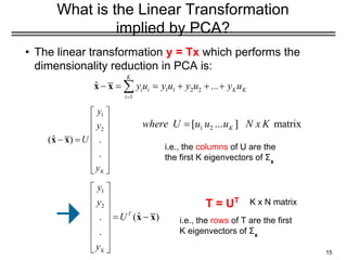
What is the Linear Transformation
implied by PCA?
• The linear transformation y = Tx which performs the
dimensionality reduction in PCA is:
i.e., the rows of T are the first
K eigenvectors of Σx
T = UT
i.e., the columns of U are the
the first K eigenvectors of Σx
K x N matrix

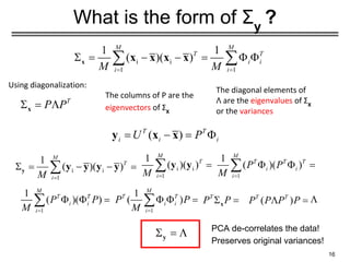
16. What is the form of Σy
?
16
The columns of P are the
eigenvectors of ΣX
The diagonal elements of
Λ are the eigenvalues of ΣX
or the variances
PCA de-correlates the data!
Preserves original variances!
Using diagonalization:

17. 17
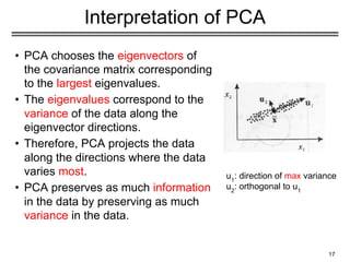
Interpretation of PCA
• PCA chooses the eigenvectors of
the covariance matrix corresponding
to the largest eigenvalues.
• The eigenvalues correspond to the
variance of the data along the
eigenvector directions.
• Therefore, PCA projects the data
along the directions where the data
varies most.
• PCA preserves as much information
in the data by preserving as much
variance in the data.
u1
: direction of max variance
u2
: orthogonal to u1

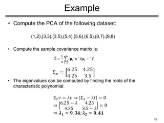
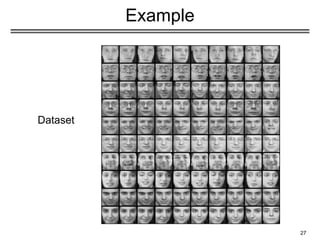
18. Example
• Compute the PCA of the following dataset:
(1,2),(3,3),(3,5),(5,4),(5,6),(6,5),(8,7),(9,8)
• Compute the sample covariance matrix is:
• The eigenvalues can be computed by finding the roots of the
characteristic polynomial:
18

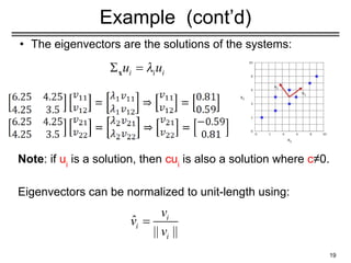
19. Example (cont’d)
• The eigenvectors are the solutions of the systems:
Note: if ui
is a solution, then cui
is also a solution where c≠0.
Eigenvectors can be normalized to unit-length using:
19

20. 20
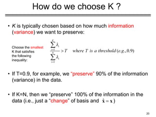
How do we choose K ?
• K is typically chosen based on how much information
(variance) we want to preserve:
• If T=0.9, for example, we “preserve” 90% of the information
(variance) in the data.
• If K=N, then we “preserve” 100% of the information in the
data (i.e., just a “change” of basis and )
Choose the smallest
K that satisfies
the following
inequality:

21. 21
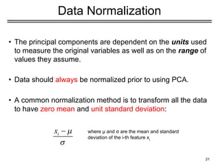
Data Normalization
• The principal components are dependent on the units used
to measure the original variables as well as on the range of
values they assume.
• Data should always be normalized prior to using PCA.
• A common normalization method is to transform all the data
to have zero mean and unit standard deviation:
where μ and σ are the mean and standard
deviation of the i-th feature xi

22. 22
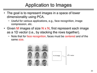
Application to Images
• The goal is to represent images in a space of lower
dimensionality using PCA.
− Useful for various applications, e.g., face recognition, image
compression, etc.
• Given M images of size N x N, first represent each image
as a 1D vector (i.e., by stacking the rows together).
− Note that for face recognition, faces must be centered and of the
same size.

23. Application to Images (cont’d)
• The key challenge is that the covariance matrix Σx
is now
very large (i.e., N2
x N2
) – see Step 3:
Step 3: compute the covariance matrix Σx
• Σx
is now an N2
x N2
matrix – computationally expensive to
compute its eigenvalues/eigenvectors λi
, ui
(AAT
)ui
= λi
ui
23
where A=[Φ1
Φ2
... ΦΜ
]
(N2
x M matrix)

24. Application to Images (cont’d)
• We will use a simple “trick” to get around this by relating
the eigenvalues/eigenvectors of AAT
to those of AT
A.
• Let us consider the matrix AT
A instead (i.e., M x M matrix)
− Suppose its eigenvalues/eigenvectors are μi
, vi
(AT
A)vi
= μi
vi
− Multiply both sides by A:
A(AT
A)vi
=Aμi
vi
or (AAT
)(Avi
)= μi
(Avi
)
− Assuming (AAT
)ui
= λi
ui
λi
=μi
and ui
=Avi
24
A=[Φ1
Φ2
... ΦΜ
]
(N2
x M matrix)

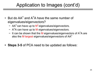
25. Application to Images (cont’d)
• But do AAT
and AT
A have the same number of
eigenvalues/eigenvectors?
− AAT
can have up to N2
eigenvalues/eigenvectors.
− AT
A can have up to M eigenvalues/eigenvectors.
− It can be shown that the M eigenvalues/eigenvectors of AT
A are
also the M largest eigenvalues/eigenvectors of AAT
• Steps 3-5 of PCA need to be updated as follows:
25

26. Application to Images (cont’d)
Step 3 compute AT
A (i.e., instead of AAT
)
Step 4: compute μi
, vi
of AT
A
Step 4b: compute λi
, ui
of AAT
using λi
=μi
and ui
=Avi
, then
normalize ui
to unit length.
Step 5: dimensionality reduction step – approximate x using
only the first K eigenvectors (K<M):
26
each image can be
represented by
a K-dimensional
vector

27. 27
Example
Dataset

28. 28
Example (cont’d)
Top eigenvectors: u1
,…uk
(visualized as an image - eigenfaces)
Mean face:
u1
u2
u3

29. 29
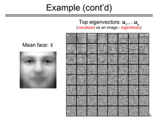
Example (cont’d)
u1
u2
u3
• How can you visualize the eigenvectors (eigenfaces)
as an image?
− Their values must be first mapped to integer values in
the interval [0, 255] (required by PGM format).
− Suppose fmin
and fmax
are the min/max values of a given
eigenface (could be negative).
− If xϵ[fmin
, fmax
] is the original value, then the new value yϵ
[0,255] can be computed as follows:
y=(int)255(x - fmin
)/(fmax
- fmin
)

30. 30
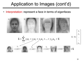
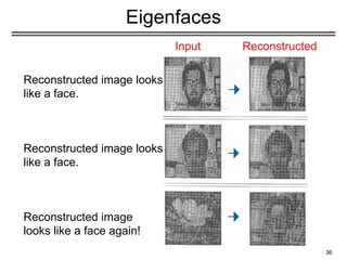
Application to Images (cont’d)
• Interpretation: represent a face in terms of eigenfaces
u1
u2
u3
y1 y2
y3

31. 31
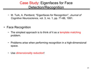
Case Study: Eigenfaces for Face
Detection/Recognition
− M. Turk, A. Pentland, "Eigenfaces for Recognition", Journal of
Cognitive Neuroscience, vol. 3, no. 1, pp. 71-86, 1991.
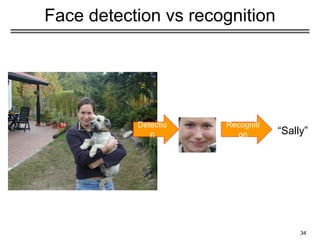
• Face Recognition
− The simplest approach is to think of it as a template matching
problem.
− Problems arise when performing recognition in a high-dimensional
space.
− Use dimensionality reduction!

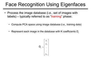
32. • Process the image database (i.e., set of images with
labels) – typically referred to as “training” phase:
− Compute PCA space using image database (i.e., training data)
− Represent each image in the database with K coefficients Ωi
Face Recognition Using Eigenfaces
Ωi

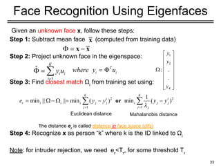
33. Given an unknown face x, follow these steps:
Step 1: Subtract mean face (computed from training data)
Step 2: Project unknown face in the eigenspace:
Step 3: Find closest match Ωi
from training set using:
Step 4: Recognize x as person “k” where k is the ID linked to Ωi
Note: for intruder rejection, we need er
<Tr
, for some threshold Tr
33
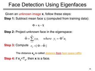
Face Recognition Using Eigenfaces
The distance er
is called distance in face space (difs)
Euclidean distance Mahalanobis distance

34. 34
Face detection vs recognition
Detectio
n
Recogniti
on “Sally”

35. Given an unknown image x, follow these steps:
Step 1: Subtract mean face (computed from training data):
Step 2: Project unknown face in the eigenspace:
Step 3: Compute
Step 4: if ed
<Td
, then x is a face.
35
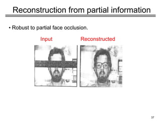
Face Detection Using Eigenfaces
The distance ed
is called distance from face space (dffs)

36. 36
Eigenfaces
Reconstructed image looks
like a face.
Reconstructed image looks
like a face.
Reconstructed image
looks like a face again!
Input Reconstructed

37. 37
Reconstruction from partial information
• Robust to partial face occlusion.
Input Reconstructed