Download as PDF, PPTX
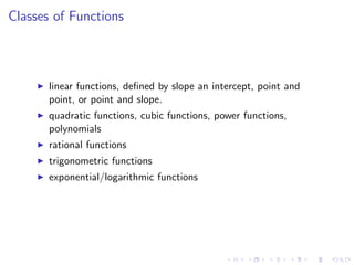
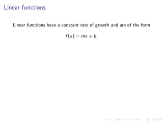
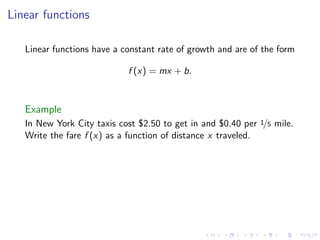
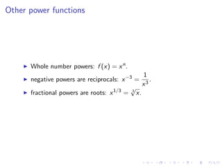
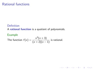
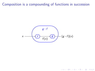
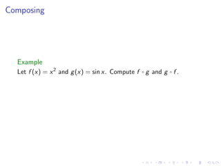
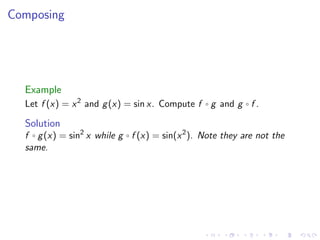
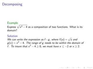

The document outlines essential functions for a Calculus I course, covering various classes of functions including linear, quadratic, cubic, rational, trigonometric, and exponential/logarithmic functions. It discusses their characteristics, transformations, and applications in modeling real-world problems. Additionally, it emphasizes the process of composing and decomposing functions with practical examples.