The document introduces a three variable analogue of Bessel polynomials. It defines the three variable Bessel polynomial c(b,a,z;y,(x,Y)),n(γ,β,α) and provides several representations. It reduces to known one and two variable Bessel polynomials under certain conditions. The polynomial has integral representations involving triple integrals over infinite intervals of products of gamma functions and powers of the variables. Laplace transformations and generating functions are also obtained.

1. International
OPEN ACCESS Journal
Of Modern Engineering Research (IJMER)
| IJMER | ISSN: 2249–6645 | www.ijmer.com | Vol. 4 | Iss. 3 | Mar. 2014 | 1 |
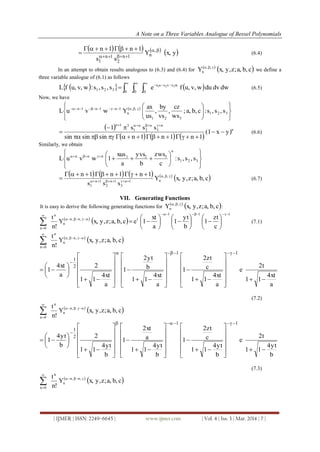
A Note on a Three Variables Analogue of Bessel Polynomials
Bhagwat Swaroop Sharma
I. Introduction
In 1949 Krall and Frink [12] initiated a study of simple Bessel polynomial





2
x
;n;1,nF(x)Y o2n (1.1)
and generalized Bessel polynomial
  




b
x
;n;1a,nFxb,a,Y o2n (1.2)
These polynomials were introduced by them in connection with the solution of the wave equation in
spherical coordinates. They are the polynomial solutions of the differential equation.
x2
y (x) + (ax + b) y (x) = n (n + a – 1) y (x) (1.3)
where n is a positive integer and a and b are arbitrary parameters. These polynomials are orthogonal on the unit
circle with respect to the weight function
n
0n x
2
)1n(
)(
i2
1
),x( 









 


. (1.4)
Several authors including Agarwal [1], Al-Salam [2], Brafman [3], Burchnall [4], Carlitz [5],
Chatterjea [6], Dickinson [7], Eweida [9], Grosswald [10], Rainville [15] and Toscano [19] have contributed to
the study of the Bessel polynomials.
Recently in the year 2000, Khan and Ahmad [11] studied two variables analogue y)(x,Y ),(
n

of the
Bessel polynomials (x)Y )(
n

defined by





2
x
;1;n,nF(x)Y o2
)(
n (1.5)
The aim of the present paper is to introduce a three variables analogue c)b,a,z;y,(x,Y ),,(
n

of (1.2) and to
obtain certain results involving the three variables Bessel polynomial c)b,a,z;y,(x,Y ),,(
n

.
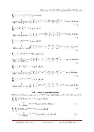
II. The Polynomials
c)b,a,z;y,(x,Y ),,(
n

: The Bessel polynomial of three variables c)b,a,z;y,(x,Y ),,(
n

is defined as
follows:
c)b,a,z;y,(x,Y ),,(
n

        rsj
rsjjsr
srn
0j
rn
0s
n
0r c
z
b
y
a
x
!j!s!r
1n1n1nn


























 (2.1)
For z = 0, a = b = 2, (2.1) reduces to the two variables analogue y)(x,Y ),(
n

of Bessel polynomials (1.5) as
given below :
y)(x,Yc)2,2,y,0;(x,Y ),(
n
),,(
n

 (2.2)
Similarly
z)(x,Yb,2)2,z;0,(x,Y ),(
n
),,(
n

 (2.3)
Abstract: The present paper deals with a study of a three variables analogue of Bessel polynomials.
Certain representations, a Schlafli’s contour integral, a fractional integral, Laplace transformations, some
generating functions and double and triple generating functions have been obtained.

2. A Note on a Three Variables Analogue of Bessel Polynomials
| IJMER | ISSN: 2249–6645 | www.ijmer.com | Vol. 4 | Iss. 3 | Mar. 2014 | 2 |
z)(y,Y2)2,a,z;y,(0,Y ),(
n
),,(
n

 (2.4)
Also for  = – n – 1, and b = c = 2
z)(y,Y2)2,a,z;y,(x,Y ),(
n
),,1n(
n

 (2.5)
Similarly,
z)(x,Y2)b,2,z;y,(x,Y ),(
n
),1n,(
n

 (2.6)
y)(x,Yc)2,2,z;y,(x,Y ),(
n
)1n,,(
n

 (2.7)
where
y)(x,Y ),(
n

     
2
y
2
x
!s!r
1n1nn
rs
rssr
rn
0s
n
0r














 


 (2.8)
Also, for y = z = 0, a = 2, (2.1) reduces to the Bessel polynomials (x)Y )(
n

as given below:
(x)Yc)b,2,0,0;(x,Y )(
n
),,(
n

 (2.9)
where (x)Y )(
n

is defined by (1.5).
Similarly
(y)Yc)2,a,0;y,(0,Y )(
n
),,(
n

 (2.10)
(z)Yc)2,2,z;0,(0,Y )(
n
),,(
n

 (2.11)
Also, for  =  = – n – 1, a = 2, we have
(x)Yc)b,2,z;y,(x,Y )(
n
)1n1,n,(
n

 (2.12)
Similarly
(y)Yc)2,a,z;y,(x,Y )(
n
)1n,1,n(
n

 (2.13)
(z)Y2)b,a,z;y,(x,Y )(
n
)1,n1,n(
n

 (2.14)
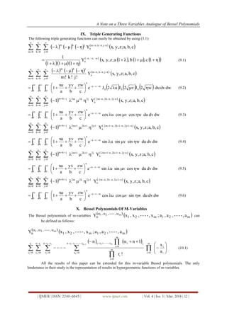
III. Integral Representations
It is easy to show that the polynomial c)b,a,z;y,(x,Y ),,(
n

has the following integral representations:
     
dwdvdue
c
zw
b
yv
a
xu
1wvu
1n1n1n
1 wvu
n
nnn
000









 
= c)b,a,z;y,(x,Y ),,(
n

(3.1)
For z = 0, a = b = 2, (3.1) reduces to
   
dvdue
2
yv
2
xu
1vu
1n1n
1 vu
n
nn
00









 
= y)(x,Y ),(
n

(3.2)
a result due to Khan and Ahmad [11].
For y = z = 0,  replaced by a – 2 and a replaced by b, (3.1) becomes
 
 
dte
b
xt
1t
n1a
1
xb,a,Y t
n
n2a
0
n










  (3.3)
a result due to Agarwal [1].
          dzdydxc,b,a;z,y,xYztzysyxrx ,,
n
1n1n1nr
0
s
0
t
0


  
     
 
 cb,a,t;s,r,Y
111
ntsr nn,n,
n
nnn
3nnn




 (3.4)
       
  dwdvduc,b,a;zwyvu,xYw1wv1vu1u ,,
n
111111
1
0
1
0
1
0



3. A Note on a Three Variables Analogue of Bessel Polynomials
| IJMER | ISSN: 2249–6645 | www.ijmer.com | Vol. 4 | Iss. 3 | Mar. 2014 | 3 |
           
      











c
z
,
b
y
,
a
x
;;;:;;::
;1,n;1,n;1,n:;;::n
F(3)
(3.5)
where F(3)
[ ] is in the form of a general triple hypergeometric series F(3)
[x, y, z]
(cf. Srivastava [18], p. 428).
       
  dwdvduc,b,a;zwyvu),1(xYw1wv1vu1u ,,
n
111111
1
0
1
0
1
0
 

           
      











c
z
,
b
y
,
a
x
;;;:;;::
;1,n;1,n;1,n:;;::n
F(3)
(3.6)
       
  dwdvduc,b,a;zw),v1(yu,xYw1wv1vu1u ,,
n
111111
1
0
1
0
1
0
 

           
      











c
z
,
b
y
,
a
x
;;;:;;::
;1,n;1,n;1,n:;;::n
F(3)
(3.7)
       
  dwdvduc,b,a);w1(z,yvu,xYw1wv1vu1u ,,
n
111111
1
0
1
0
1
0
 

           
      











c
z
,
b
y
,
a
x
;;;:;;::
;1,n;1,n;1,n:;;::n
F(3)
(3.8)
       
  dwdvduc,b,a;zw),v1(y,)u1(xYw1wv1vu1u ,,
n
111111
1
0
1
0
1
0
 

           
      











c
z
,
b
y
,
a
x
;;;:;;::
;1,n;1,n;1,n:;;::n
F(3)
(3.9)
       
  dwdvduc,b,a);w1(z,yv,)u1(xYw1wv1vu1u ,,
n
111111
1
0
1
0
1
0
 

           
      











c
z
,
b
y
,
a
x
;;;:;;::
;1,n;1,n;1,n:;;::n
F(3)
(3.10)
       
  dwdvduc,b,a);w1(z),v1(y,xuYw1wv1vu1u ,,
n
111111
1
0
1
0
1
0
 

           
      











c
z
,
b
y
,
a
x
;;;:;;::
;1,n;1,n;1,n:;;::n
F(3)
(3.11)
       
  dwdvduc,b,a);w1(z),v1(y,)u1(xYw1wv1vu1u ,,
n
111111
1
0
1
0
1
0
 

           
      











c
z
,
b
y
,
a
x
;;;:;;::
;1,n;1,n;1,n:;;::n
F(3)
(3.12)
          dwdvduc,b,a;zuv,yuw,xvwYw1wv1vu1u ,,
n
1111111
0
1
0
1
0


           
      











c
z
,
b
y
,
a
x
;;;:;;::
;1n1;n1;n:;;::n
F(3)
(3.13)

4. A Note on a Three Variables Analogue of Bessel Polynomials
| IJMER | ISSN: 2249–6645 | www.ijmer.com | Vol. 4 | Iss. 3 | Mar. 2014 | 4 |
       
 dudvdwc,b,a);v1(zu),u1(yw,)w1(xvYw1wv1vu1u ,,
n
111111
1
0
1
0
1
0
 

           
      











c
z
,
b
y
,
a
x
;;;:;;::
;,1,n;,1,n;,1,n:;;::n
F(3)
(3.14)
Particular Cases:
Some interesting particular cases of the above results are as follows :
(i) Taking  =  + 1,  =  + 1,  =  + 1,  =  =  = n in (3.5), we obtain
          dwdvduc,b,a;zwyvu,xYw1wv1vu1u ,,
n
1n1n1n1
0
1
0
1
0


  
     
 
 cb,a,z;y,x,Y
111
n nn,n,
n
nnn
3



 (3.15)
which is equivalent to (3.4)
(ii) Taking  =  =  = n + 1,  = ,  = ,  =  in (3.5), we get
       
  dwdvduzwyvu,xYw1wv1vu1u ,,
n
1n1n1n
1
0
1
0
1
0


 
     
 
 zy,x,Y
!n 0,0,0
n
1n1n1n
3
 
 (3.16)
(iii) Replacing  by  + n + 1 – ,  by  + n + 1 – ,  by  + n + 1 – , and putting  = ,  =  and  =  in
(3.5), we get
          dwdvduc,b,a;zwyvu,xYw1wv1vu1u ,,
n
1n1n1n1
0
1
0
1
0


           
     
 
 cb,a,z;y,x,Y
1n1n1n
1n1n1n ,,
n




(3.17)
Similar particular cases hold for (3.6), (3.7), (3.8), (3.9), (3.10), (3.11) and (3.12).
(iv) For z = 0, a = b = 2, results (3.4), (3.5), (3.6), (3.7) and (3.9) become
        dydxy,xYysyxrx ,
n
1n1nr
0
s
0


  
   
 
 sr,Y
11
ntsr nn,
n
nn
2nnn




 (3.18)
     
  dvduyvu,xYv1vu1u ,
n
1111
1
0
1
0


       
    










 
2
y
,
2
x
;;:
;1,n;1,n:n
F 2;2:1
1;1: (3.19)
     
  dvduyvu),1(xYv1vu1u ,
n
1111
1
0
1
0
 

       
    










 
2
y
,
2
x
;;:
;1,n;1,n:n
F 2;2:1
1;1: (3.20)
     
  dvdu)v1(yu),1(xYv1vu1u ,
n
1111
1
0
1
0
 

       
    










 
2
y
,
2
x
;;:
;1,n;1,n:n
F 2;2:1
1;1: (3.21)

5. A Note on a Three Variables Analogue of Bessel Polynomials
| IJMER | ISSN: 2249–6645 | www.ijmer.com | Vol. 4 | Iss. 3 | Mar. 2014 | 5 |
Results (3.18), (3.19), (3.20) and (3.21) are due to Khan and Ahmad [11].
Also, using the integral (see Erdelyi et al. [8], vol. I, p. 14),
    dtetzzsini2 t1z)(0


  (3.22)
and the fact that
 
 
!j!s!r
zyxn
zyx1
rsj
jsr
srn
0j
rn
0s
n
0r
n 





  (3.23)
we can easily derive the following integral representations for
 
 cb,a,;zy,x,Y ,,
n

:
      dwdvdu
c
zw
b
yv
a
xu
1ewvu
n
wvunnn)0()0()0(






 




 
         
 cb,a,;zy,x,Y1n1n1nsinsinsin1i8 ,,
n
n 

(3.24)
       
3
1n
n1n1n1sinsinsin1

 
  dwdvducb,a,;
w
cz
,
v
by
,
u
ax
Yewvu ,,
n
wvu1n1n1n
000







 n
zyx1  (3.25)
IV. Schlafli’s Contour Integral
It is easy to show that
dwdvdu
c
zw
b
yv
a
xu
1ewvu
n
wvunnn
)0()0()0(












 
         
 cb,a,;zy,x,Yn1n1n1sinsinsin1i8 ,,
n
n 

(4.1)
Proof of (4.1) : We have
 
dwdvdu
c
zw
b
yv
a
xu
1ewvu
i2
1
n
wvunnn
)0()0()0(
3 













 
 
 
dwdvduewvu
i2
1
c
z
b
y
a
x
!j!s!r
n wvurnsnjn
)0()0()0(
3
rsj
jsr
srn
0j
rn
0s
n
0r












 



















 
     rnsnjn!j!s!r
c
z
b
y
a
x
n
rsj
jsrsrn
0j
rn
0s
n
0r 

























using Hankel’s formula (see A. Eerdelyi et al. [8], 1.6 (2)).
 
dtte
i2
1
z
1 zt
)(0





(4.2)
Finally (4.1) follows from (2.1) after using the result
    zcosecz1z  (4.3)
for z = 0, a = b = 2, (4.1) reduces to
dvdu
b
yv
a
xu
1evu
n
wvunn)0()0(









 
       yx,Yn1n1sinsin4 ,
n

 (4.4)
which is due to Khan and Ahmad [11].

6. A Note on a Three Variables Analogue of Bessel Polynomials
| IJMER | ISSN: 2249–6645 | www.ijmer.com | Vol. 4 | Iss. 3 | Mar. 2014 | 6 |
V. Fractional Integrals
Let L denote the linear space of (equivalent classes of) complex – valued functions f(x) which are Lebesgue –
integrable on [0, ],  < . For f(x) L and complex number  with Rl  > 0, the Riemann – Liouville
fractional integral of order  is defined as (see Prabhakar [13], p. 72)
 
  dt(t)ftx
1
f(x)I
1x
0



  for almost all x  [0, ] (5.1)
Using the operator I
, Prabhakar [14] obtained the following result for Rl  > 0 and Rl  > –1.
    
 
 kx;Zx
1kn
1kn
kx;ZxI nn



 (5.2)
where  kx;Zn

is Konhauser’s biorthozonal polynomial.
Khan and Ahmad [11] defined a two variable analogue of (5.1) by means of the following relation :
  
   
      dvduvu,fvyux
1
yx,fI 11y
0
x
0
, 


  (5.3)
and obtained the following result :
 
  yx,YyxI ,
n
nn,     
   
 
 yx,Y
1n1n
1n1nyx ,
n
nn





(5.4)
In an attempt to obtained a result analogous to (5.4) for the polynomial
 
 cb,a,;zy,x,Y ,,
n

we
first seek a three variable analogue of (5.1).
A three variable analogue of I
may be defined as
  
     
        dwdvduwv,u,fwzvyux
1
zy,x,fI 111z
0
y
0
x
0
,, 


 
(5.5)
Putting    
 cb,a,z;y,x,Yzyxzy,,xf ,,
n
nnn 
 in (5.5), we obtain
 
  cb,a,z;y,x,YzyxI ,,
n
nnn,, 

     
     
 
 cb,a,z;y,x,Y
1n1n1n
1n1n1nzyx ,,
n
nnn





(5.6)
VI. Laplace Transform
In the usual notation the Laplace transform is given by
       0asRldt,tfes:tfL st
0
 

 (6.1)
where f  L (0, R) for every R > 0 and f(t) = 0(eat
), t  .
Khan and Ahmad [11] introduced a two variable analogue of (6.1) by means of the relation:
     dvduvu,fes,s:vu,fL vsus
00
21
21 

 (6.2)
and established the following results :
 












21
21
,
n
1n1n
s,s:
vs
2y
,
us
2x
YvuL
   
 n
n
2
n
1
2
yx1
1n1nsinsin
ss





(6.3)
and















21
n
21nn
s,s:
2
yvs
2
xus
1vuL

7. A Note on a Three Variables Analogue of Bessel Polynomials
| IJMER | ISSN: 2249–6645 | www.ijmer.com | Vol. 4 | Iss. 3 | Mar. 2014 | 7 |
       yx,Y
ss
1n1n ,
n1n
2
1n
1



 (6.4)
In an attempt to obtain results analogous to (6.3) and (6.4) for
 
 cb,a,z;y,x,Y ,,
n

we define a
three variable analogue of (6.1) as follows
     dwdvduwv,u,fes,s,s:wv,u,fL wsvsus
000
321
321 
 (6.5)
Now, we have
 












321
321
,,
n
1n1n1n
s,s,s:cb,a,;
ws
cz
,
vs
by
,
us
ax
YwvuL
 
     
n
n
3
n
2
n
1
31n
y)x(1
1n1n1nsinsinsin
sss1





(6.6)
Similarly, we obtain















321
n
321nnn
s,s,s:
c
zws
b
yvs
a
xus
1wvuL
       
 cb,a,z;y,x,Y
sss
1n1n1n ,,
n1n
3
1n
2
1n
1



 (6.7)
VII. Generating Functions
It is easy to derive the following generating functions for
 
 cb,a,z;y,x,Y ,,
n

:
 
 
111
tn,n,n
n
n
0n c
zt
1
b
yt
1
a
xt
1ecb,a,z;y,x,Y
!n
t






















 (7.1)
 
 cb,a,z;y,x,Y
!n
t n,n,
n
n
0n




a
xt4
11
t2
e
a
xt4
11
c
zt2
1
a
xt4
11
b
yt2
1
a
xt4
11
2
a
xt4
1
11
2
1


















































(7.2)
 
 cb,a,z;y,x,Y
!n
t n,,n
n
n
0n




b
yt4
11
t2
e
b
yt4
11
c
zt2
1
b
yt4
11
a
xt2
1
b
yt4
11
2
b
yt4
1
11
2
1


















































(7.3)
 
 cb,a,z;y,x,Y
!n
t ,n,n
n
n
0n





8. A Note on a Three Variables Analogue of Bessel Polynomials
| IJMER | ISSN: 2249–6645 | www.ijmer.com | Vol. 4 | Iss. 3 | Mar. 2014 | 8 |
c
zt4
11
t2
11
2
1
e
c
zt4
11
b
yt2
1
c
zt4
11
a
xt2
1
c
zt4
11
2
c
zt4
1


















































 (7.4)
 
 cb,a,z;y,x,Y
!n
t n,n,n2
n
n
0n




   
11
xta
at
xtac
azt
1
xtab
ayt
1
a
xt
1e























 (7.5)
 
 cb,a,z;y,x,Y
!n
t n,n2,n
n
n
0n




   
11
ytb
bt
ytbc
bzt
1
ytba
bxt
1
b
yt
1e























 (7.6)
 
 cb,a,z;y,x,Y
!n
t n2,n,n
n
n
0n




   
11
ztc
ct
ztcb
cyt
1
ztca
cxt
1
c
zt
1e























 (7.7)
   
   
  1cb,a,z;y,x,Y
1
1
cb,a,z;y,x,Y n,,
n
nk,,
n
k
0k


 


 (7.8)
          c,1ba,z;y,x,Y
1
1
cb,a,z;y,x,Y ,n,
n
,nk,
n
k
0k


 


 (7.9)
          c,b,1az;y,x,Y
1
1
cb,a,z;y,x,Y ,,n
n
,,nk
n
k
0k


 


 (7.10)
Using (3.1), we can also derive the following results :
   
 cb,a,z;y,x,Y
!k
nk,,
n
k
0k





   
  dwdvduw2Je
c
zw
b
yv
a
xu
1vu
1n1n
1
0
wvu
n
nn
000








 


(7.11)
   
 cb,a,z;y,x,Y
!k
,nk,
n
k
0k





   
  dwdvduv2Je
c
zw
b
yv
a
xu
1wu
1n1n
1
0
wvu
n
nn
000








 


(7.12)
   
 cb,a,z;y,x,Y
!k
,,nk
n
k
0k





   
  dwdvduu2Je
c
zw
b
yv
a
xu
1wu
1n1n
1
0
wvu
n
nn
000








 


(7.13)

9. A Note on a Three Variables Analogue of Bessel Polynomials
| IJMER | ISSN: 2249–6645 | www.ijmer.com | Vol. 4 | Iss. 3 | Mar. 2014 | 9 |
   
 cb,a,z;y,x,Y1 n2k,,
n
2kk
0k




   
dwdvduwosce
c
zw
b
yv
a
xu
1vu
1n1n
1 wvu
n
nn
000








 


(7.14)
   
 cb,a,z;y,x,Y1 ,n2k,
n
k2k
0k




   
dwdvduvosce
c
zw
b
yv
a
xu
1wu
1n1n
1 wvu
n
nn
000








 


(7.15)
   
 cb,a,z;y,x,Y1 ,,n2k
n
2kk
0k




   
dwdvduuosce
c
zw
b
yv
a
xu
1wu
1n1n
1 wvu
n
nn
000








 


(7.16)
   
 cb,a,z;y,x,Y1 n12k,,
n
12kk
0k




   
dwdvduwsine
c
zw
b
yv
a
xu
1vu
1n1n
1 wvu
n
nn
000








 


(7.17)
   
 cb,a,z;y,x,Y1 ,n12k,
n
1k2k
0k




   
dwdvduvsine
c
zw
b
yv
a
xu
1wu
1n1n
1 wvu
n
nn
000








 


(7.18)
   
 cb,a,z;y,x,Y1 ,,n12k
n
12kk
0k




   
dwdvduusine
c
zw
b
yv
a
xu
1wu
1n1n
1 wvu
n
nn
000








 


(7.19)
VIII. Double Generating Functions
The following double generating functions for
 
 cb,a,z;y,x,Y ,,
n

can easily be derived by using (3.1)
     
 cb,a,z;y,x,Y ,nk,nm
n
km
0k0m






  
 
    c,1b,1a;zy,,xY
11
1 n,n,
n 

 
(8.1)
     
 cb,a,z;y,x,Y nk,,nm
n
km
0k0m






  
 
    

 
1cb,,1a;zy,,xY
11
1 n,n,
n (8.2)

10. A Note on a Three Variables Analogue of Bessel Polynomials
| IJMER | ISSN: 2249–6645 | www.ijmer.com | Vol. 4 | Iss. 3 | Mar. 2014 | 10 |
     
 cb,a,z;y,x,Y nk,nm,
n
km
0k0m






  
 
    

 
1c,1ba,;zy,,xY
11
1 nn,,
n
(8.3)
     
 cb,a,z;y,x,Y
!k!m
,nk,nm
n
km
0k0m







 
    dwdvduv2Ju2Je
c
zw
b
yv
a
xu
1w
1n
1
00
wvu
n
n
000








 


(8.4)
     
 cb,a,z;y,x,Y
!k!m
nk,,nm
n
km
0k0m







 
    dwdvduw2Ju2Je
c
zw
b
yv
a
xu
1v
1n
1
00
wvu
n
n
000








 


(8.5)
     
 cb,a,z;y,x,Y
!k!m
nk,nm,
n
km
0k0m







 
    dwdvduw2Jv2Je
c
zw
b
yv
a
xu
1u
1n
1
00
wvu
n
n
000








 

(8.6)
   
 cb,a,z;y,x,Y1 ,n2k,nm2
n
2k2mkm
0k0m






 
dwdvduvcosuosce
c
zw
b
yv
a
xu
1w
1n
1 wvu
n
n
000








 

(8.7)
   
 cb,a,z;y,x,Y1 n2k,,nm2
n
2k2mkm
0k0m






 
dwdvduwcosuosce
c
zw
b
yv
a
xu
1v
1n
1 wvu
n
n
000








 


(8.8)
   
 cb,a,z;y,x,Y1 n2k,nm2,
n
2k2mkm
0k0m






 
dwdvduwcosvosce
c
zw
b
yv
a
xu
1u
1n
1 wvu
n
n
000








 


(8.9)
   
 cb,a,z;y,x,Y1 ,n2k,n1m2
n
2k12mkm
0k0m






 
dwdvduvcosuinse
c
zw
b
yv
a
xu
1w
1n
1 wvu
n
n
000








 


(8.10)
   
 cb,a,z;y,x,Y1 n2k,,n1m2
n
2k12mkm
0k0m







11. A Note on a Three Variables Analogue of Bessel Polynomials
| IJMER | ISSN: 2249–6645 | www.ijmer.com | Vol. 4 | Iss. 3 | Mar. 2014 | 11 |
 
dwdvduwcosuinse
c
zw
b
yv
a
xu
1v
1n
1 wvu
n
n
000








 

(8.11)
   
 cb,a,z;y,x,Y1 n2k,n1m2,
n
2k12mkm
0k0m






 
dwdvduwcosvinse
c
zw
b
yv
a
xu
1u
1n
1 wvu
n
n
000








 

(8.12)
   
 cb,a,z;y,x,Y1 ,n12k,nm2
n
12k2mkm
0k0m






 
dwdvduvsinuosce
c
zw
b
yv
a
xu
1w
1n
1 wvu
n
n
000








 


(8.13)
   
 cb,a,z;y,x,Y1 n12k,,nm2
n
12k2mkm
0k0m






 
dwdvduwsinuosce
c
zw
b
yv
a
xu
1v
1n
1 wvu
n
n
000








 


(8.14)
   
 cb,a,z;y,x,Y1 n12k,nm2,
n
12k2mkm
0k0m






 
dwdvduwsinvosce
c
zw
b
yv
a
xu
1u
1n
1 wvu
n
n
000








 


(8.15)
   
 cb,a,z;y,x,Y1 ,n12k,n1m2
n
12k12mkm
0k0m






 
dwdvduvsinuinse
c
zw
b
yv
a
xu
1w
1n
1 wvu
n
n
000








 


(8.16)
   
 cb,a,z;y,x,Y1 n12k,,n1m2
n
12k12mkm
0k0m






 
dwdvduwsinuinse
c
zw
b
yv
a
xu
1v
1n
1 wvu
n
n
000








 


(8.17)
   
 cb,a,z;y,x,Y1 n12k,n1m2,
n
12k12mkm
0k0m






 
dwdvduwsinvinse
c
zw
b
yv
a
xu
1u
1n
1 wvu
n
n
000








 


(8.18)

12. A Note on a Three Variables Analogue of Bessel Polynomials
| IJMER | ISSN: 2249–6645 | www.ijmer.com | Vol. 4 | Iss. 3 | Mar. 2014 | 12 |
IX. Triple Generating Functions
The following triple generating functions can easily be obtained by using (3.1):
       
 cb,a,z;y,x,Y nj,nk,nm
n
jkm
0j0k0m








   
 
      

 
1c,1b,1az;y,x,Y
111
1 n,n,n
n (9.1)
       
 cb,a,z;y,x,Y
!j!k!m
nj,nk,nm
n
jkm
0j0k0m









      dwdvduw2Jv2Ju2Je
c
zw
b
yv
a
xu
1 000
wvu
n
000






 

 (9.2)
   
 cb,a,z;y,x,Y1 n2j,n2k,nm2
n
2j2k2mjkm
0j0k0m








dwdvduwoscvoscuosce
c
zw
b
yv
a
xu
1 wvu
n
000






 

 (9.3)
   
 cb,a,z;y,x,Y1 n12j,n12k,n1m2
n
12j12k12mjkm
0j0k0m








dwdvduwinsvinsuinse
c
zw
b
yv
a
xu
1 wvu
n
000






 

 (9.4)
   
 cb,a,z;y,x,Y1 n2j,n12k,n1m2
n
2j12k12mjkm
0j0k0m








dwdvduwoscvinsuinse
c
zw
b
yv
a
xu
1 wvu
n
000






 

 (9.5)
   
 cb,a,z;y,x,Y1 n12j,n2k,nm2
n
12j2k2mjkm
0j0k0m








dwdvduwinsvoscuosce
c
zw
b
yv
a
xu
1 wvu
n
000






 

 (9.6)
X. Bessel Polynomials Of M-Variables
The Bessel polynomials of m-variables
   m21m21
,----,,
n a,----,a,a;x,----,x,xY m21 
can
be defined as follows:
   m21m21
,----,,
n a,----,a,a;x,----,x,xY m21 
   








 


 









i
i
m
0i
i
m
0i
ji
m
0i
rrrrrrn
0r
rrn
0r
rn
0r
n
0r a
x
!r
1nn m211m21
m
21
3
1
21
(10.1)
All the results of this paper can be extended for this m-variable Bessel polynomials. The only
hinderance in their study is the representation of results in hypergeometric functions of m-variables.

13. A Note on a Three Variables Analogue of Bessel Polynomials
| IJMER | ISSN: 2249–6645 | www.ijmer.com | Vol. 4 | Iss. 3 | Mar. 2014 | 13 |
REFERENCES
[1.] R. P. Agarwal: On Bessel polynomials, Canadian Journal of Mathematics, Vol. 6 (1954), pp. 410 – 415.
[2.] W. A. Al-Salam: On Bessel polynomials, Duke Math. J., Vol. 24 (1957), pp. 529 – 545.
[3.] F.Brafman: A set of generating functions for Bessel polynomials, Proc. Amer. Math Soc., Vol. 4 (1953), pp. 275
– 277.
[4.] J. L. Burchnall: The Bessel polynomials, Canadian Journal of Mathematics, Vol. 3 (1951), pp 62 – 68.
[5.] L. Carlitz: On the Bessel polynomials, Duke Math. Journal, Vol. 24 (1957), pp. 151 – 162.
[6.] S. K. Chatterjea: Some generating functions, Duke Math. Journal, Vol. 32 (1965), pp. 563 – 564.
[7.] D. Dickinson: On Lommel and Bessel polynomials, Proc. Amar. Math. Soc., Vol. 5 (1954), pp. 946 – 956.
[8.] A. Erdelyi et. al: Higher Transcendal Functions, I, McGraw Hill, New York (1953).
[9.] M. T. Eweida: On Bessel polynomials, Math. Zeitsehr., Vol. 74 (1960), pp. 319 – 324.
[10.] E. Grosswald: On some algebraic properties of the Bessel polynomials, Trans. Amer. Math. Soc., Vol. 71 (1951),
pp. 197 – 210.
[11.] M. A. Khan and K. Ahmad: On a two variables analogue of Bessel polynomials, Mathematica Balkanica, New
series Vol. 14, (2000), Fasc. 1 – 2, pp. 65 – 76.
[12.] H. L. Krall: and O. Frink A new class of orthogonal polynomials, the Bessel polynomials, Trans. Amer. Math.
Soc., Vol. 65 (1949), pp. 100 – 115.
[13.] T. R. Prabhakar: Two singular integral equations involving confluent hypergeometric functions, Proc. Camb.
Phil. Soc., Vol. 66 (1969), pp. 71 – 89.
[14.] T. R. Prabhakar: On a set of polynomials suggested by Laguerre polynomials, Pacific Journal of Mathematics,
Vol. 40 (1972), pp. 311 – 317.
[15.] E. D. Rainville: Generating functions for Bessel and related polynomials, Canadian J. Math., Vol. 5 (1953), pp.
104 – 106.
[16.] E. D. Rainville: Special Functions, MacMillan, New York, Reprinted by Chelsea Publ. Co., Bronx – New York
(1971).
[17.] H. M. Srivastava: Some biorthogonal polynomials suggested by the Laguerre polynomials, Pacific J. Math., Vol.
98, No. 1 (1982), pp. 235 – 249.
[18.] H. M. Srivastava and H. L. Masnocha: A treatise on Generating Functions, J. Waley & Sons (Halsted Press), New
York; Ellis Horwood, Chichester (1984).
[19.] L. Toscano: Osservacioni e complementi su particolari polinomiipergeometrici, Le Matematiche, Vol. 10 (1955),
pp. 121 – 133.