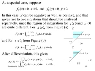
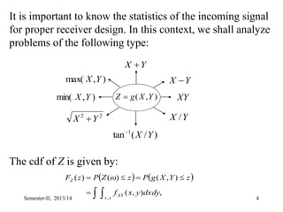
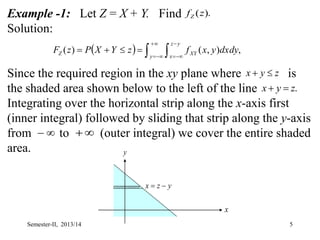
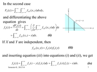
Chapter 3: Multiple Random Variables
Addis Ababa Science & Technology University
Department of Electrical & Electronics Engineering
Probability and Random Process (EEEg-2114)
Multiple Random Variables
Outline
 Introduction
 The Joint Cumulative Distribution Function
 The Joint Probability Density and Mass Functions
 Marginal Statistics
 Independence
 Conditional Distributions
 Correlation and Covariance
 Functions of Two Random Variables
Semester-II, 2013/14 2
3
One Function of Two Random Variables
Given two random variables X and Y and a function g(x,y),
we form a new random variable Z as
Given the joint pdf how does one obtain
the pdf of Z ? Problems of this type are of interest from a
practical standpoint. For example, a receiver output signal
usually consists of the desired signal buried in noise, and
the above formulation in that case reduces to Z = X + Y.
).
,
( Y
X
g
Z 
),
,
( y
x
fXY ),
(z
fZ
Semester-II, 2013/14
4
It is important to know the statistics of the incoming signal
for proper receiver design. In this context, we shall analyze
problems of the following type:
The cdf of Z is given by:
)
,
( Y
X
g
Z 
Y
X 
)
/
(
tan 1
Y
X

Y
X 
XY
Y
X /
)
,
max( Y
X
)
,
min( Y
X
2
2
Y
X 
   
 





y
x
XY
Z
dxdy
y
x
f
z
Y
X
g
P
z
Z
P
z
F
,
,
)
,
(
)
,
(
)
(
)
( 
Semester-II, 2013/14
5
Example -1: Let Z = X + Y. Find
Solution:
Since the required region in the xy plane where is
the shaded area shown below to the left of the line
Integrating over the horizontal strip along the x-axis first
(inner integral) followed by sliding that strip along the y-axis
from to (outer integral) we cover the entire shaded
area.
   










 ,
)
,
(
)
(
y
y
z
x
XY
Z dxdy
y
x
f
z
Y
X
P
z
F
z
y
x 

.
z
y
x 


 

y
z
x 

x
y
).
(z
fZ
Semester-II, 2013/14
6
We can find by differentiating directly. In this
context, it is useful to recall the differentiation rule by
Leibnitz. Suppose
Then,
Using the above two equations, we get
Alternatively, the above integration can be carried out first
along the y-axis followed by the x-axis as below.
)
(z
FZ
)
(z
fZ


)
(
)
(
.
)
,
(
)
(
z
b
z
a
dx
z
x
h
z
H
     




)
(
)
(
.
)
,
(
),
(
)
(
),
(
)
(
)
( z
b
z
a
dx
z
z
x
h
z
z
a
h
dz
z
da
z
z
b
h
dz
z
db
dz
z
dH
( , )
( ) ( , ) ( , ) 0
( , ) .
z y z y
XY
Z XY XY
XY
f x y
f z f x y dx dy f z y y dy
z z
f z y y dy
   
   



  
 
    
   
 
   
 
   
 (i)
Semester-II, 2013/14
7
In the second case
and differentiating the above
equation gives
 







 ,
)
,
(
)
(
x
x
z
y
XY
Z dxdy
y
x
f
z
F

 























.
)
,
(
)
,
(
)
(
)
(
x
XY
x
x
z
y
XY
Z
Z
dx
x
z
x
f
dx
dy
y
x
f
z
dz
z
dF
z
f
(ii)
If X and Y are independent, then
and inserting equation (iii) into equations (i) and (ii), we get
)
(
)
(
)
,
( y
f
x
f
y
x
f Y
X
XY 
.
)
(
)
(
)
(
)
(
)
( 













x
Y
X
y
Y
X
Z dx
x
z
f
x
f
dy
y
f
y
z
f
z
f
(iii)
(iv)
x
z
y 

x
y
Semester-II, 2013/14
8
The above integral is the standard convolution of the
functions and expressed two different ways. We
thus reach the following conclusion: If two random variables
are independent, then the density of their sum equals the
convolution of their density functions.
As a special case, suppose that for and
for then we can use the following figure to determine
the pdf of Z.
)
(z
fX )
(z
fY
0
)
( 
x
fX 0

x 0
)
( 
y
fY
,
0

y
y
z
x 

x
y
)
0
,
(z
)
,
0
( z
Semester-II, 2013/14
9
In the above case,
or
On the other hand, by considering vertical strips first in
above figure, we get
or
if X and Y are independent random variables.
 




z
y
y
z
x
XY
Z dxdy
y
x
f
z
F
0 0
)
,
(
)
(

















 
 



.
0
,
0
,
0
,
)
,
(
)
,
(
)
( 0
0 0
z
z
dy
y
y
z
f
dy
dx
y
x
f
z
z
f
z
XY
z
y
y
z
x
XY
Z










 
 

,
0
,
0
,
0
,
)
(
)
(
)
,
(
)
( 0
0
z
z
dx
x
z
f
x
f
dx
x
z
x
f
z
f
z
y
Y
X
z
x
XY
Z
 




z
x
x
z
y
XY
Z dydx
y
x
f
z
F
0 0
)
,
(
)
(
Semester-II, 2013/14
10
Example-2: Suppose X and Y are independent exponential
r.vs with common parameter , and let Z = X + Y.
Determine
Solution: We have
and we can make use of (13) to obtain the pdf of Z = X + Y.
As the next example shows, care should be taken in using
the convolution formula for r.vs with finite range.
Example-3: X and Y are independent uniform r.vs in the
common interval (0,1). Determine where Z = X + Y.
Solution: Clearly, here, and as following
figure shows there are two cases of z for which the shaded
areas are quite different in shape and they should be
considered separately.
),
(
)
(
),
(
)
( y
U
e
y
f
x
U
e
x
f y
Y
x
X



 



2
0 



 z
Y
X
Z
),
(z
fZ
).
(
)
( 2
0
2
0
)
(
2
z
U
e
z
dx
e
dx
e
e
z
f z
z
z
z
x
z
x
Z






 






 

).
(z
fZ
Semester-II, 2013/14
11
x
y
y
z
x 

1
0
)
( 
 z
a
x
y
y
z
x 

2
1
)
( 
 z
b
For
For notice that it is easy to deal with the unshaded
region. In that case
,
1
0 
 z
,
2
1 
 z
.
1
0
,
2
)
(
1
)
(
2
0
0 0





 
  



z
z
dy
y
z
dxdy
z
F
z
y
z
y
y
z
x
Z
 
.
2
1
,
2
)
2
(
1
)
1
(
1
1
1
1
)
(
2
1
1
z
1
1
1















 



 

z
z
dy
y
z
dxdy
z
Z
P
z
F
y
z
y y
z
x
Z
Semester-II, 2013/14
12
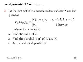
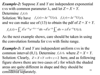
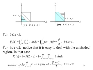
Finally, differentiating the cdf, we obtain
By direct convolution of and we obtain the
same result as above. In fact, for [Figure (a)]
and for [Figure (b)]
Figure (c) shows which agrees with the convolution
of two rectangular waveforms as well.










.
2
1
,
2
,
1
0
)
(
)
(
z
z
z
z
dz
z
dF
z
f Z
Z
)
(x
fX ),
( y
fY
1
0 
 z
2
1 
 z
.
1
)
(
)
(
)
(
0
z
dx
dx
x
f
x
z
f
z
f
z
Y
X
Z 


  
.
2
1
)
(
1
1
z
dx
z
f
z
Z 

  
)
(z
fZ
Semester-II, 2013/14
13
)
(x
fY
x
1
)
( x
z
fX 
x
z
)
(
)
( x
f
x
z
f Y
X 
x
z
1

z
1
0
)
( 
 z
a
)
(x
fY
x
1
)
( x
z
fX 
x
)
(
)
( x
f
x
z
f Y
X 
x
1
1

z z
1

z
2
1
)
( 
 z
b
(c)
)
(z
fZ
z
2
0 1
Semester-II, 2013/14
14
Example-4: Let Determine its pdf
Solution:
and hence
If X and Y are independent, then the above formula reduces
to
which represents the convolution of with
.
Y
X
Z 

   










 )
,
(
)
(
y
y
z
x
XY
Z dxdy
y
x
f
z
Y
X
P
z
F
( )
( ) ( , ) ( , ) .
z y
Z
Z XY XY
y x
dF z
f z f x y dx dy f y z y dy
dz z
  
  

 
   
 

 
  
( ) ( ) ( ) ( ) ( ),
Z X Y X Y
f z f z y f y dy f z f y


    

)
( z
fX  ).
(z
fY
y
x
z
y
x 

z
y
x 

y
).
(z
fZ
Semester-II, 2013/14
15
As a special case, suppose
In this case, Z can be negative as well as positive, and that
gives rise to two situations that should be analyzed
separately, since the region of integration for and
are quite different. For from Figure (a)
and for from Figure (b)
After differentiation, this gives
 






0 0
)
,
(
)
(
y
y
z
x
XY
Z dxdy
y
x
f
z
F
 







0
)
,
(
)
(
z
y
y
z
x
XY
Z dxdy
y
x
f
z
F
.
0
,
0
)
(
and
,
0
,
0
)
( 


 y
y
f
x
x
f Y
X
0

z 0

z
,
0

z
,
0

z

















.
0
,
)
,
(
,
0
,
)
,
(
)
( 0
z
dy
y
y
z
f
z
dy
y
y
z
f
z
f
z
XY
XY
Z
(b)
y
x
y
z
x 

z

y
x
y
z
x 

z
z

(a)
Semester-II, 2013/14
16
Example-5: Given Z = X / Y, obtain its density function.
Solution: We have
The inequality can be rewritten as if
and if
Figure (a) shows the area corresponding to the first term,
and Figure (b) shows that corresponding to the second term
in the above equation.
 .
/
)
( z
Y
X
P
z
FZ 

z
Y
X 
/ Yz
X  ,
0

Y
Yz
X  .
0

Y
y
x
yz
x 
(a)
y
x
yz
x 
(b)
     
   .
0
,
0
,
0
,
/
0
,
/
/













Y
Yz
X
P
Y
Yz
X
P
Y
z
Y
X
P
Y
z
Y
X
P
z
Y
X
P
Semester-II, 2013/14
17
Integrating over these two regions, we get
Differentiation with respect to z gives
Note that if X and Y are nonnegative random variables, then
the area of integration reduces to that shown below
.
)
,
(
)
,
(
)
(
0
0  
  





 



y yz
x
XY
y
yz
x
XY
Z dxdy
y
x
f
dxdy
y
x
f
z
F
.
,
)
,
(
|
|
)
,
(
)
(
)
,
(
)
(
0
0




















z
dy
y
yz
f
y
dy
y
yz
f
y
dy
y
yz
yf
z
f
XY
XY
XY
Z
y
x
yz
x 
Semester-II, 2013/14
Exercise
The joint pdf of two random variables X and Y is given by:
Find the pdf of Z if :
otherwise
,
0
1
0
,
1
0
,
)
,
(


 





y
x
y
x
y
x
fXY
18
Y
X
Z
d
Y
X
Z
b
XY
Z
c
Y
X
Z
a






.
.
.
.
Semester-II, 2013/14
Assignment-III
1. Suppose that two continuous random variables X and Y have
joint pdf given by:
)
2
0
(
.
)
3
(
.
)
4
(
.
)
2
,
4
3
(
.
ies.
probabilit
following
the
Evaluate
.
.
and
of
pdf
l
conditiona
the
Find
.
t?
independen
and
Are
.
.
and
of
pdf
and
cdf
marginal
the
Find
.
.
and
of
cdf
joint
the
Find
.
.
constant
the
Find
.
constant.
a
is
re
whe
otherwise
,
0
5
0
,
6
2
,
)
2
(
)
,
(










 





Y
P
iv
X
P
ii
Y
X
P
iii
Y
X
P
i
e
Y
X
e
Y
X
d
Y
X
c
Y
X
b
k
a
k
y
x
y
x
k
y
x
fXY
Semester-II, 2013/14 19
Assignment-III Cont’d……
2. Let the joint pmf of two discrete random variables X and Y is
given by:
t?
independen
and
Are
.
.
and
of
pmf
marginal
the
Find
.
.
of
value
the
Find
.
constant.
a
is
re
whe
otherwise
,
0
2
,
1
3;
2,
,
1
,
)
(
)
,
(
Y
X
c
Y
X
b
k
a
k
y
x
y
x
k
y
x
P
i
j
i
j
i
XY


 



Semester-II, 2013/14 20
Assignment-III Cont’d…..
3. Suppose that two continuous random variables X and Y are
independent and uniform in the interval (0, 4).
Find the pdf of Z if :
.
.
.
.
.
X
Y
Z
e
XY
Z
d
Y
X
Z
c
X
Y
Z
b
Y
X
Z
a








21
Semester-II, 2013/14

03probability nd statistics -Multiple Random Variables-II.ppt

  • 1.
    Chapter 3: MultipleRandom Variables Addis Ababa Science & Technology University Department of Electrical & Electronics Engineering Probability and Random Process (EEEg-2114)
  • 2.
    Multiple Random Variables Outline Introduction  The Joint Cumulative Distribution Function  The Joint Probability Density and Mass Functions  Marginal Statistics  Independence  Conditional Distributions  Correlation and Covariance  Functions of Two Random Variables Semester-II, 2013/14 2
  • 3.
    3 One Function ofTwo Random Variables Given two random variables X and Y and a function g(x,y), we form a new random variable Z as Given the joint pdf how does one obtain the pdf of Z ? Problems of this type are of interest from a practical standpoint. For example, a receiver output signal usually consists of the desired signal buried in noise, and the above formulation in that case reduces to Z = X + Y. ). , ( Y X g Z  ), , ( y x fXY ), (z fZ Semester-II, 2013/14
  • 4.
    4 It is importantto know the statistics of the incoming signal for proper receiver design. In this context, we shall analyze problems of the following type: The cdf of Z is given by: ) , ( Y X g Z  Y X  ) / ( tan 1 Y X  Y X  XY Y X / ) , max( Y X ) , min( Y X 2 2 Y X             y x XY Z dxdy y x f z Y X g P z Z P z F , , ) , ( ) , ( ) ( ) (  Semester-II, 2013/14
  • 5.
    5 Example -1: LetZ = X + Y. Find Solution: Since the required region in the xy plane where is the shaded area shown below to the left of the line Integrating over the horizontal strip along the x-axis first (inner integral) followed by sliding that strip along the y-axis from to (outer integral) we cover the entire shaded area.                , ) , ( ) ( y y z x XY Z dxdy y x f z Y X P z F z y x   . z y x       y z x   x y ). (z fZ Semester-II, 2013/14
  • 6.
    6 We can findby differentiating directly. In this context, it is useful to recall the differentiation rule by Leibnitz. Suppose Then, Using the above two equations, we get Alternatively, the above integration can be carried out first along the y-axis followed by the x-axis as below. ) (z FZ ) (z fZ   ) ( ) ( . ) , ( ) ( z b z a dx z x h z H           ) ( ) ( . ) , ( ), ( ) ( ), ( ) ( ) ( z b z a dx z z x h z z a h dz z da z z b h dz z db dz z dH ( , ) ( ) ( , ) ( , ) 0 ( , ) . z y z y XY Z XY XY XY f x y f z f x y dx dy f z y y dy z z f z y y dy                                       (i) Semester-II, 2013/14
  • 7.
    7 In the secondcase and differentiating the above equation gives           , ) , ( ) ( x x z y XY Z dxdy y x f z F                           . ) , ( ) , ( ) ( ) ( x XY x x z y XY Z Z dx x z x f dx dy y x f z dz z dF z f (ii) If X and Y are independent, then and inserting equation (iii) into equations (i) and (ii), we get ) ( ) ( ) , ( y f x f y x f Y X XY  . ) ( ) ( ) ( ) ( ) (               x Y X y Y X Z dx x z f x f dy y f y z f z f (iii) (iv) x z y   x y Semester-II, 2013/14
  • 8.
    8 The above integralis the standard convolution of the functions and expressed two different ways. We thus reach the following conclusion: If two random variables are independent, then the density of their sum equals the convolution of their density functions. As a special case, suppose that for and for then we can use the following figure to determine the pdf of Z. ) (z fX ) (z fY 0 ) (  x fX 0  x 0 ) (  y fY , 0  y y z x   x y ) 0 , (z ) , 0 ( z Semester-II, 2013/14
  • 9.
    9 In the abovecase, or On the other hand, by considering vertical strips first in above figure, we get or if X and Y are independent random variables.       z y y z x XY Z dxdy y x f z F 0 0 ) , ( ) (                         . 0 , 0 , 0 , ) , ( ) , ( ) ( 0 0 0 z z dy y y z f dy dx y x f z z f z XY z y y z x XY Z                , 0 , 0 , 0 , ) ( ) ( ) , ( ) ( 0 0 z z dx x z f x f dx x z x f z f z y Y X z x XY Z       z x x z y XY Z dydx y x f z F 0 0 ) , ( ) ( Semester-II, 2013/14
  • 10.
    10 Example-2: Suppose Xand Y are independent exponential r.vs with common parameter , and let Z = X + Y. Determine Solution: We have and we can make use of (13) to obtain the pdf of Z = X + Y. As the next example shows, care should be taken in using the convolution formula for r.vs with finite range. Example-3: X and Y are independent uniform r.vs in the common interval (0,1). Determine where Z = X + Y. Solution: Clearly, here, and as following figure shows there are two cases of z for which the shaded areas are quite different in shape and they should be considered separately. ), ( ) ( ), ( ) ( y U e y f x U e x f y Y x X         2 0      z Y X Z ), (z fZ ). ( ) ( 2 0 2 0 ) ( 2 z U e z dx e dx e e z f z z z z x z x Z                  ). (z fZ Semester-II, 2013/14
  • 11.
    11 x y y z x   1 0 ) (  z a x y y z x   2 1 ) (   z b For For notice that it is easy to deal with the unshaded region. In that case , 1 0   z , 2 1   z . 1 0 , 2 ) ( 1 ) ( 2 0 0 0              z z dy y z dxdy z F z y z y y z x Z   . 2 1 , 2 ) 2 ( 1 ) 1 ( 1 1 1 1 ) ( 2 1 1 z 1 1 1                        z z dy y z dxdy z Z P z F y z y y z x Z Semester-II, 2013/14
  • 12.
    12 Finally, differentiating thecdf, we obtain By direct convolution of and we obtain the same result as above. In fact, for [Figure (a)] and for [Figure (b)] Figure (c) shows which agrees with the convolution of two rectangular waveforms as well.           . 2 1 , 2 , 1 0 ) ( ) ( z z z z dz z dF z f Z Z ) (x fX ), ( y fY 1 0   z 2 1   z . 1 ) ( ) ( ) ( 0 z dx dx x f x z f z f z Y X Z       . 2 1 ) ( 1 1 z dx z f z Z      ) (z fZ Semester-II, 2013/14
  • 13.
    13 ) (x fY x 1 ) ( x z fX  x z ) ( ) (x f x z f Y X  x z 1  z 1 0 ) (   z a ) (x fY x 1 ) ( x z fX  x ) ( ) ( x f x z f Y X  x 1 1  z z 1  z 2 1 ) (   z b (c) ) (z fZ z 2 0 1 Semester-II, 2013/14
  • 14.
    14 Example-4: Let Determineits pdf Solution: and hence If X and Y are independent, then the above formula reduces to which represents the convolution of with . Y X Z                  ) , ( ) ( y y z x XY Z dxdy y x f z Y X P z F ( ) ( ) ( , ) ( , ) . z y Z Z XY XY y x dF z f z f x y dx dy f y z y dy dz z                      ( ) ( ) ( ) ( ) ( ), Z X Y X Y f z f z y f y dy f z f y         ) ( z fX  ). (z fY y x z y x   z y x   y ). (z fZ Semester-II, 2013/14
  • 15.
    15 As a specialcase, suppose In this case, Z can be negative as well as positive, and that gives rise to two situations that should be analyzed separately, since the region of integration for and are quite different. For from Figure (a) and for from Figure (b) After differentiation, this gives         0 0 ) , ( ) ( y y z x XY Z dxdy y x f z F          0 ) , ( ) ( z y y z x XY Z dxdy y x f z F . 0 , 0 ) ( and , 0 , 0 ) (     y y f x x f Y X 0  z 0  z , 0  z , 0  z                  . 0 , ) , ( , 0 , ) , ( ) ( 0 z dy y y z f z dy y y z f z f z XY XY Z (b) y x y z x   z  y x y z x   z z  (a) Semester-II, 2013/14
  • 16.
    16 Example-5: Given Z= X / Y, obtain its density function. Solution: We have The inequality can be rewritten as if and if Figure (a) shows the area corresponding to the first term, and Figure (b) shows that corresponding to the second term in the above equation.  . / ) ( z Y X P z FZ   z Y X  / Yz X  , 0  Y Yz X  . 0  Y y x yz x  (a) y x yz x  (b)          . 0 , 0 , 0 , / 0 , / /              Y Yz X P Y Yz X P Y z Y X P Y z Y X P z Y X P Semester-II, 2013/14
  • 17.
    17 Integrating over thesetwo regions, we get Differentiation with respect to z gives Note that if X and Y are nonnegative random variables, then the area of integration reduces to that shown below . ) , ( ) , ( ) ( 0 0                y yz x XY y yz x XY Z dxdy y x f dxdy y x f z F . , ) , ( | | ) , ( ) ( ) , ( ) ( 0 0                     z dy y yz f y dy y yz f y dy y yz yf z f XY XY XY Z y x yz x  Semester-II, 2013/14
  • 18.
    Exercise The joint pdfof two random variables X and Y is given by: Find the pdf of Z if : otherwise , 0 1 0 , 1 0 , ) , (          y x y x y x fXY 18 Y X Z d Y X Z b XY Z c Y X Z a       . . . . Semester-II, 2013/14
  • 19.
    Assignment-III 1. Suppose thattwo continuous random variables X and Y have joint pdf given by: ) 2 0 ( . ) 3 ( . ) 4 ( . ) 2 , 4 3 ( . ies. probabilit following the Evaluate . . and of pdf l conditiona the Find . t? independen and Are . . and of pdf and cdf marginal the Find . . and of cdf joint the Find . . constant the Find . constant. a is re whe otherwise , 0 5 0 , 6 2 , ) 2 ( ) , (                  Y P iv X P ii Y X P iii Y X P i e Y X e Y X d Y X c Y X b k a k y x y x k y x fXY Semester-II, 2013/14 19
  • 20.
    Assignment-III Cont’d…… 2. Letthe joint pmf of two discrete random variables X and Y is given by: t? independen and Are . . and of pmf marginal the Find . . of value the Find . constant. a is re whe otherwise , 0 2 , 1 3; 2, , 1 , ) ( ) , ( Y X c Y X b k a k y x y x k y x P i j i j i XY        Semester-II, 2013/14 20
  • 21.
    Assignment-III Cont’d….. 3. Supposethat two continuous random variables X and Y are independent and uniform in the interval (0, 4). Find the pdf of Z if : . . . . . X Y Z e XY Z d Y X Z c X Y Z b Y X Z a         21 Semester-II, 2013/14