This paper investigates the dynamical behavior of a discrete model of one prey two predator systems. The equilibrium points and their stability are analyzed. Time series plots are obtained for different sets of parameter values. Also bifurcation diagrams are plotted to show dynamical behavior of the system in selected range of growth parameter

1. International
OPEN ACCESS Journal
Of Modern Engineering Research (IJMER)
| IJMER | ISSN: 2249–6645 | www.ijmer.com | Vol. 5 | Iss.3| Mar. 2015 | 49|
Discrete Model of Two Predators competing for One Prey
A. George Maria Selvam1
, P. Rathinavel2
, J. MariaThangaraj3
1,2
Sacred Heart College, Tirupattur - 635 601, S.India.
3
Thiruvalluvar University College of Arts and Science, Gajalnaickanpatti, S.India
I. INTRODUCTION
Ecology is the study of inter-relationships between organisms and environment. It is natural that two
or more species living in a common habitat interact in different ways. The application of mathematics to
ecology dates back to the book “An Essay on the Principle of Population” by Malthus. In recent decades, many
researchers [1,2] have focused on the ecological models with three and more species to understand complex
dynamical behaviors of ecological systems in the real world. They have demonstrated very complex dynamic
phenomena of those models, including cycles, periodic doubling and chaos [6,7]. The discrete time models
which are usually described by difference equations produce much richer patterns [3, 4, 5]. Discrete time
models are ideally suited to describe the population dynamics of species, which are characterized by discrete
generations.
II. MATHEMATICAL MODEL
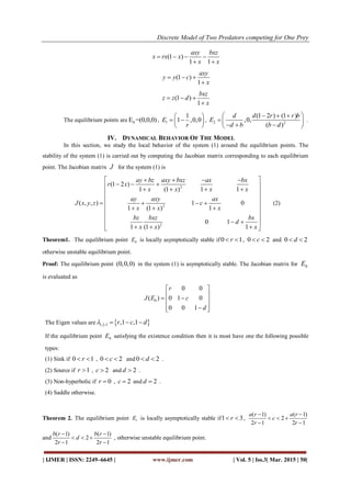
In this paper, we consider the one prey- two predator systems describing the interactions among three
species by the following system of difference equations:
( ) ( ) ( ) ( )
( 1) ( )(1 ( ))
1 ( ) 1 ( )
ax n y n bx n z n
x n rx n x n
x n x n
    
 
( ) ( )
( 1) ( )(1 )
1 ( )
ax n y n
y n y n c
x n
   

(1)
( ) ( )
( 1) ( )(1 )
1 ( )
bx n z n
z n z n d
x n
   

where ( )x n Prey, ( )y n and ( )z n are two predator respectively, and all parameters are positive constants.
The parameter a is the intrinsic growth rates of the prey population, b denotes the death rate of the mid-
predator, c denotes the death rate of the top predator, d is the rate of conversion of a consumed prey to a
mid-predator, e is the rate of conversion of a consumed mid-predator to a top predator.
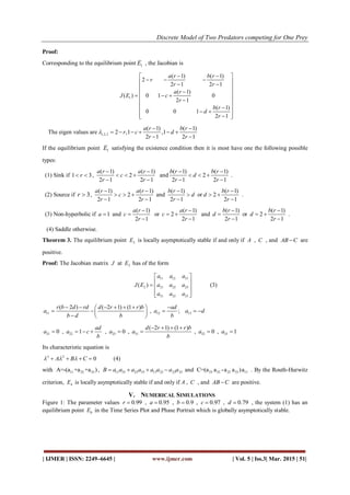
III. EXISTENCE OF EQUILIBRIUM
The equilibrium points of (1) are the solution of the equations
ABSTRACT: This paper investigates the dynamical behavior of a discrete model of one prey two
predator systems. The equilibrium points and their stability are analyzed. Time series plots are obtained
for different sets of parameter values. Also bifurcation diagrams are plotted to show dynamical behavior
of the system in selected range of growth parameter.
Keywords: Discrete Model, Prey - Predator System, Equilibrium Points, Local Stability, Time Plots,
Bifurcation.

2. Discrete Model of Two Predators competing for One Prey
| IJMER | ISSN: 2249–6645 | www.ijmer.com | Vol. 5 | Iss.3| Mar. 2015 | 50|
(1 )
1 1
axy bxz
x rx x
x x
   
 
(1 )
1
axy
y y c
x
  

(1 )
1
bxz
z z d
x
  

The equilibrium points are 0E =(0,0,0), 1
1
1 ,0,0E
r
 
  
 
, 2 2
(1 2 ) (1 )
,0,
( )
d d r r b
E
d b b d
   
  
   
.
IV. DYNAMICAL BEHAVIOR OF THE MODEL
In this section, we study the local behavior of the system (1) around the equilibrium points. The
stability of the system (1) is carried out by computing the Jacobian matrix corresponding to each equilibrium
point. The Jacobian matrix J for the system (1) is
2
2
2
(1 2 )
1 (1 ) 1 1
( , , ) 1 0
1 (1 ) 1
0 1
1 (1 ) 1
ay bz axy bxz ax bx
r x
x x x x
ay axy ax
J x y z c
x x x
bz bxz bx
d
x x x
    
       
 
    
   
 
  
   
(2)
Theorem1. The equilibrium point 0E is locally asymptotically stable if0 1r  , 0 2c  and 0 2d 
otherwise unstable equilibrium point.
Proof: The equilibrium point (0,0,0) in the system (1) is asymptotically stable. The Jacobian matrix for 0E
is evaluated as
0
0 0
( ) 0 1 0
0 0 1
r
J E c
d
 
   
  
The Eigen values are  1,2,3 ,1 ,1r c d   
If the equilibrium point 0E satisfying the existence condition then it is most have one the following possible
types:
(1) Sink if 0 1r  , 0 2c  and 0 2d  .
(2) Source if 1r  , 2c  and 2d  .
(3) Non-hyperbolic if 0r  , 2c  and 2d  .
(4) Saddle otherwise.
Theorem 2. The equilibrium point 1E is locally asymptotically stable if1 3r  ,
( 1) ( 1)
2
2 1 2 1
a r a r
c
r r
 
  
 
and
( 1) ( 1)
2
2 1 2 1
b r b r
d
r r
 
  
 
, otherwise unstable equilibrium point.

3. Discrete Model of Two Predators competing for One Prey
| IJMER | ISSN: 2249–6645 | www.ijmer.com | Vol. 5 | Iss.3| Mar. 2015 | 51|
Proof:
Corresponding to the equilibrium point 1E , the Jacobian is
1
( 1) ( 1)
2
2 1 2 1
( 1)
( ) 0 1 0
2 1
( 1)
0 0 1
2 1
a r b r
r
r r
a r
J E c
r
b r
d
r
  
    
 
   
 
 
  
  
The eigen values are 1,2,3
( 1) ( 1)
2 ,1 ,1
2 1 2 1
a r b r
r c d
r r

 
     
 
If the equilibrium point 1E satisfying the existence condition then it is most have one the following possible
types:
(1) Sink if 1 3r  ,
( 1) ( 1)
2
2 1 2 1
a r a r
c
r r
 
  
 
and
( 1) ( 1)
2
2 1 2 1
b r b r
d
r r
 
  
 
.
(2) Source if 3r  ,
( 1) ( 1)
2
2 1 2 1
a r a r
c
r r
 
  
 
and
( 1)
2 1
b r
d
r



or
( 1)
2
2 1
b r
d
r

 

.
(3) Non-hyperbolic if 1a  and
( 1)
2 1
a r
c
r



or
( 1)
2
2 1
a r
c
r

 

and
( 1)
2 1
b r
d
r



or
( 1)
2
2 1
b r
d
r

 

.
(4) Saddle otherwise.
Theorem 3. The equilibrium point 2E is locally asymptotically stable if and only if A , C , and AB C are
positive.
Proof: The Jacobian matrix J at 2E has of the form
11 12 13
2 21 22 23
31 32 33
( )
a a a
J E a a a
a a a
 
   
  
(3)
11
( 2 ) ( 2 1) (1 )r b d rd d r r b
a
b d b
      
  
  
, 12 13;
ad
a a d
b

  
21 0a  , 22 1
ad
a c
b
   , 23 0a  , 31
( 2 1) (1 )d r r b
a
b
   
 , 32 0a  , 33 1a 
Its characteristic equation is
3 2
0A B C      (4)
with 11 22 33A=-(a +a +a ), 11 33 22 33 11 22 23 32B a a a a a a a a    and 23 32 22 33 11C=(a a -a a )a . By the Routh-Hurwitz
criterion, 4E is locally asymptotically stable if and only if A , C , and AB C are positive.
V. NUMERICAL SIMULATIONS
Figure 1: The parameter values 0.99r  , 0.95a  , 0.9b  , 0.97c  , 0.79d  , the system (1) has an
equilibrium point 0E in the Time Series Plot and Phase Portrait which is globally asymptotically stable.

4. Discrete Model of Two Predators competing for One Prey
| IJMER | ISSN: 2249–6645 | www.ijmer.com | Vol. 5 | Iss.3| Mar. 2015 | 52|
Fig 1. Time Series Plot and Phase Portrait at E0
Figure 2: The parameter values r=2.89, a=0.9, b=1.35, c=0.99, d=1.09, the system (1) has a equilibrium point
E1 in the Time Series Plot and Phase Portrait which is globally asymptotically stable.
Fig 2. Time Series Plot and Phase Portrait at E1
Figure 3: The parameter values r=1.98, a=1.78, b=0.41, c=0.94, d=0.09, the system (1) has a equilibrium point
2E in the Time Series Plot and Phase Portrait which is globally asymptotically stable.
Fig 3. Time Series Plot and Phase Portrait at E2
VI. BIFURCATION
Bifurcation is a change of the dynamical behaviours of the system as its parameters pass through a
bifurcation (critical) value. Bifurcation usually occurs when the stability of an equilibrium changes. An

5. Discrete Model of Two Predators competing for One Prey
| IJMER | ISSN: 2249–6645 | www.ijmer.com | Vol. 5 | Iss.3| Mar. 2015 | 53|
examination of the bifurcation diagram of the system shows that a given qualitative change in the functioning
of the ecosystem may be produced by changing different parameters. We restrict our analysis to events that
occur when the parameter a is changed, and the other parameters are fixed at given values. In this section, we
focus on exploring the possibility of chaotic behaviour for the prey population respectively.
Fig 4. Bifurcation diagram for prey population
Variation of prey population

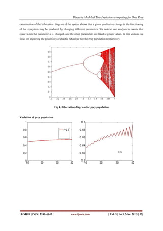
6. Discrete Model of Two Predators competing for One Prey
| IJMER | ISSN: 2249–6645 | www.ijmer.com | Vol. 5 | Iss.3| Mar. 2015 | 54|
Fig 5. Variation of prey population
REFERENCES
Journal Papers:
[1]. Abd-Elalim A. Elsadany, Dynamical complexities in a discrete-time food chain, Computational
Ecology and Software, 2012, 2(2):124-139.
[2]. Sophia R. -J. Jang, Jui- Ling Yu, Models of plant quality and larch budmoth interaction, Nonlinear
Analysis(2009), doi: 10.1016/.na.2009.02.091.
[3]. Debasis Mukherjee, Prasenjit Das & Dipak Kesh, Dynamics of a Plant-Herbivore Model with Holling
Type II Functional Response.
[4]. A. George Maria Selvam, R. Dhineshbabu, and V.Sathish, Dynamical Behavior in a Discrete Three
Species Prey-Predator System, International Journal of Innovative Science, Engineering & Technology
(IJISET), Volume 1, Issue 8, October 2014, ISSN: 2348-7968, pp 335 - 339.
[5]. A. George Maria Selvam, R. Janagaraj, P. Rathinavel, A Discrete Model of Three Species Prey-
Predator System, International Journal of Innovative Research in Science, Engineering & Technology,
ISSN (Online): 2319-8753, ISSN (Print): 2347-6710, Vol. 4, Issue 1, January 2015, DOI:
10.15680/IJIRSET.2015.0401023, pp: 18576 to 18584.
[6]. Prasenjit Das, Debasis Mukherjee & Kalyan Das, Chaos in a Prey- Predator Model with infection in
Predator- A Parameter Domain Analysis, Computational and Mathematical Biology.
Books:
[7]. Saber Elaydi, An Introduction to Difference Equations, Third Edition, Springer International Edition,
First Indian Reprint, 2008.