Download to read offline
![The Limiting Absorption Principle for the
Elasticity Operator in Homogeneous
Anisotropic Media
Alejandro Domínguez-Torres1
Abstract
The spectral theory is studied and the principle of limiting absorption is proved for the elasticity operator
derived from the wave equations in infinite elastic homogeneous anisotropic media.
The Wave Equation for Elastic Homogeneous Anisotropic Media
For a medium obeying the generalized Hooke´s Law, the linear stress-strain relations in rectangular
Cartesian coordinates xi ; i 1,2,3; are [Achenbach p. 52 and Fedorov pp. 8-9]
(1) ij Cijlm lm ; i , j , l , m 1,2,3.
Here ij is the stress tensor, lm is the strain tensor, and C ijlm are the elastic coefficients satisfying the
symmetry conditions [Achenbach p. 52 and Fedorov pp. 12-15]:
(2) Cijlm C jilm Cijml Clmij .
In this way, only 21 independent constants are involved. Moreover, the convention summation for
repeated suffixes is assumed.
The strain tensor may be expressed in terms of the displacement vector ui ; i 1,2,3; by
1 u u
(3) ij i j .
2 x j xi
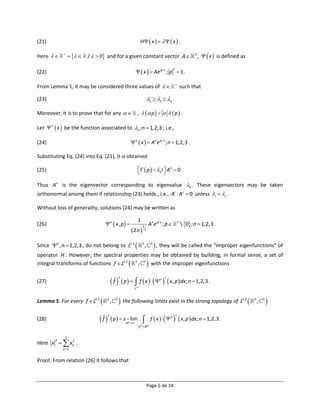
In the absence of body forces and considering that the density of the medium is constant and equal to
one, the equation of motions are [Fedorov pp. 85-86]
2ui 2um
(4) C ijlm .
t 2 x j xl
It is also assumed that the constants C ijlm have numerical values such that the strain energy W is
positive definite for symmetric stress components ij ji , where:
1
This research paper is derived from the thesis dissertation (Spectral Theory for Elasticity Equations) presented
th
(August 24 , 1989) by the author for obtaining the degree of Master of Science (Physics) at the School of Sciences
in the Universidad Nacional Autónoma de México. This paper never was published.
Page 1 de 14](https://image.slidesharecdn.com/thelimitingabsorptionprinciplefortheelasticequations-101230014515-phpapp02/85/The-limiting-absorption-principle-for-the-elastic-equations-1-320.jpg)
![The Limiting Absorption Principle for the
Elasticity Operator in Homogeneous
Anisotropic Media
Alejandro Domínguez-Torres1
Abstract
The spectral theory is studied and the principle of limiting absorption is proved for the elasticity operator
derived from the wave equations in infinite elastic homogeneous anisotropic media.
The Wave Equation for Elastic Homogeneous Anisotropic Media
For a medium obeying the generalized Hooke´s Law, the linear stress-strain relations in rectangular
Cartesian coordinates xi ; i 1,2,3; are [Achenbach p. 52 and Fedorov pp. 8-9]
(1) ij Cijlm lm ; i , j , l , m 1,2,3.
Here ij is the stress tensor, lm is the strain tensor, and C ijlm are the elastic coefficients satisfying the
symmetry conditions [Achenbach p. 52 and Fedorov pp. 12-15]:
(2) Cijlm C jilm Cijml Clmij .
In this way, only 21 independent constants are involved. Moreover, the convention summation for
repeated suffixes is assumed.
The strain tensor may be expressed in terms of the displacement vector ui ; i 1,2,3; by
1 u u
(3) ij i j .
2 x j xi
In the absence of body forces and considering that the density of the medium is constant and equal to
one, the equation of motions are [Fedorov pp. 85-86]
2ui 2um
(4) C ijlm .
t 2 x j xl
It is also assumed that the constants C ijlm have numerical values such that the strain energy W is
positive definite for symmetric stress components ij ji , where:
1
This research paper is derived from the thesis dissertation (Spectral Theory for Elasticity Equations) presented
th
(August 24 , 1989) by the author for obtaining the degree of Master of Science (Physics) at the School of Sciences
in the Universidad Nacional Autónoma de México. This paper never was published.
Page 1 de 14](https://image.slidesharecdn.com/thelimitingabsorptionprinciplefortheelasticequations-101230014515-phpapp02/75/The-limiting-absorption-principle-for-the-elastic-equations-1-2048.jpg)
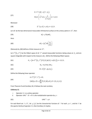
![3
f x n x , p dx
1 1
(29) 2 f x Ane ipx dx f j x e ipx dx An .
j 1 2 2
j
2 2
3 3
2 2 2
x M2 x M x M2
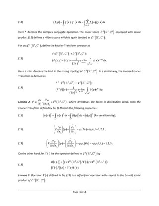
Since A n are constants for j 1,2,3 ; and fj L2
j , then from the Plancharel’s Theorem [Bochner 3
,
and Chandrasekaran pp.112-113] it follows that the integral (29) converges in the norm of L , and 2 3
the limit belongs to the same linear space.
For f L2,3 3
, 3
, Lemma 5 associates to it a vector f 1
, f 2 , f 3 , where f n L2 3
, , n 1,2,3 .
Moreover, the following result holds.
Lemma 6. For each f L2,3 3
, 3
, it follows the Parseval Identity
3
fn
2 2
(30) f .
n 1
L2 3
,
Here f n , n 1,2,3 ; are defined by expression (28).
Proof. From relations (26) and (27) it follows that
(31) ˆ ˆ ˆ ˆ
f n f A1 , f A2 , f A3 fA ;
ˆ
where A is a 3 3 matrix whose columns are formed by An , n 1,2,3 ; and f Ff . Moreover, A is an
orthogonal matrix since its columns are orthonormal vector, thus A1 A† .
On the other hand,
3 3 3 3
fn, fn f n p dp f p f p fˆ p A
2 2 2 2 2
fn n
dp dp
n 1
2
L 3
, n 1
2
L 3
, n 1 3 3 n 1 3 3
fˆ p f x
2 2 2
dp dx f .
3 3
The previous to last equality follows from Parseval’s identity for Fourier Transforms [Bochner and
Chandrasekaran p. 113].
Define the following linear operator
: L2,3 L 3
, 3 2,3 3
, 3
(32)
f f f , f , f . 1 2 3
Therefore, from Lemma 6 the next identity holds
(33) f f , f L2,3 3
, 3
.
This means that
Page 6 de 14](https://image.slidesharecdn.com/thelimitingabsorptionprinciplefortheelasticequations-101230014515-phpapp02/85/The-limiting-absorption-principle-for-the-elastic-equations-6-320.jpg)
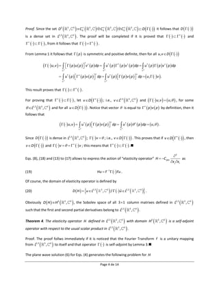
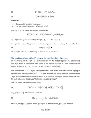
![(34) I .
Therefore is a partial isometry and P is the orthogonal projection of L2,3 3
, 3
, the
range of .
(35)
f f A1 , f A2 , f A3 ; f L2,3
ˆ ˆ ˆ 3
, 3
.
ˆ
This means that the components of f are the projections of f on each An ; n 1,2,3 . Therefore, the
vector base formed by An ; n 1,2,3 ; vector f may be expressed as
f f An An ; f L2,3
3
(36) ˆ 3
, 3
n 1
From this interpretation and from Plancherel´s Theorem [Bochner and Chandrasekaran pp.112-113] it is
obtained the following result.
Lemma 7. For each f L2,3 3
, 3
, the following limits exist on For each L 2,3 3
, 3
.
3
f s lim f p x , p dp .
n
(37) n
M
p M2 n 1
2
Here fn ; n 1,2,3 ; are the components of f .
From Eq. (37), it may be seen that
(38) f F 1 Af .
Theorem 8. The operator defined in (32) is a unitary linear operator; i.e.,
(39) I .
Proof. The first equality of (39) follows from (34). On the other hand, since A is orthonormal, then it is
the matrix of a bijective linear transformation. Thus, if f L2,3 3 , 3 then g Af L2,3 3 , 3 .
Moreover, since F is a unitary linear transformation from L2,3 3
, 3
to itself, then F 1
g L2,3 3
, 3
.
Therefore, if h f ,
(40) f f h h† A .
ˆ
From Eq. (38) it follows that
h† f FF 1 Af Af fA† .
† † †
(41) ˆ
Combination of Eqs. (40) and (41) gives
f fA† A fI f .
Page 7 de 14](https://image.slidesharecdn.com/thelimitingabsorptionprinciplefortheelasticequations-101230014515-phpapp02/85/The-limiting-absorption-principle-for-the-elastic-equations-7-320.jpg)
![Eq. (39) is the eigenfunction expansion in abstract form; i.e., for each, it follows the next representation
(42) f f .
This eigenfunction expansion may be used to obtain a representation for the elasticity operator H .
Theorem 9. The operator whose action is given by Eqs. (32), (35), and (36) defines a spectral
representation for H in the sense
(43)
Hf 1 f 1 , 2 f 2 , 3 f 3 ; f D H .
Proof. Since D3 3
, 3
C
0
3
, C
0
3
, C
0
3
, is a dense set on L2,3 3
, 3
, thus if
f D H and g D3 , then
3
Hf , g Hf , g F Ff ,F Ag Ff ,FF Ag Ff , Ag
1 1 1
(44)
A Ff , g A IFf , g A AA Ff , g A Af , g .
† † † † †
Matrix A† A is a diagonal matrix whose components are the eigenvalues of :
(45) A† A i ij .
Thus Eq. (44) becomes
(46) Hf , g A Af , g f , g .
†
Eq. (43) follows immediately from Eq (46) since D3 3
, 3
is a dense set on L 2,3 3
, 3
.
Notice that Eq. (43) implies that
(47) H .
This means that operator diagonalizes operator H .
Let Pn be the orthogonal projection on the corresponding eigenspace of n ; n 1,2,3 . Then Pn is
given by [Kato]
1 dz
(48) Pn p p p z ; n 1,2,3 .
2 i Cn
Here C n p is a simple closed curve around n p ; n 1,2,3 . From Lemma 6, Lemma 7, Theorem 8, and
Theorem 9, the following corollary is proved.
Corollary 10. Operators , H , and Pn hold the following properties on L2,3 3
, 3
Page 8 de 14](https://image.slidesharecdn.com/thelimitingabsorptionprinciplefortheelasticequations-101230014515-phpapp02/85/The-limiting-absorption-principle-for-the-elastic-equations-8-320.jpg)
![3
(49) P p I; p
n 1
n
3
0 ;
3
(50) p A n p Pn p A† ; p 3
0 ;
n 1
3 3
(51) H F 1 A n p Pn p A† n p Pn p ; p 3
0 ;
n 1 n 1
3
(52) P I; P
n 1
n n Pn .
In order to find out more properties of the spectrum of the elasticity operator, return to Christoffel
equation (9) and its corresponding associated equation (10). For a fixed , Eq. (10) defines a two-
dimensional surface on the vector spaced defined by vector p . Since the second term in Eq. (10) is
p
proportional to 2 and p p1 , p2 , p3 3 0 , with p p1 p2 p3 1 ; let q 1 be the
2 2 2 2
2
2 1
“slowness vector” [Achenbach p. 126], then it follows that q . In this way and in virtue of Eq. (8),
Eq. (9) becomes
p I u C ijlm pl pm im u C ijlm ql qm im u C ijlmql qm im u 0 .
This last equation in turn implies that
(53) 1, q q I 0 .
Eq. (53) describes an inverse velocity two-dimensional surface known in literature as “slowness surface”.
1
Notice that this surface is independent of 2
and only depends on the direction of propagation
vector q .
An alternative way of describing the slowness surface is by noticing that Eq. (53) is a polynomial of third
degree that in turn may be factorized in a unique way as
(54) 1, q Q1 1, q Q2 1, q Q3 1, q 0 .
The locus described by each Qn 1, q ; n 1,2,3 ; is given by the following set
(55) Sn 3
/ n 1; n 1,2,3 .
Therefore, the slowness surface is given by
3
(56) S Sn .
n 1
This description for the slowness surface permits defining a system of generalized radial coordinates on
3
:
Page 9 de 14](https://image.slidesharecdn.com/thelimitingabsorptionprinciplefortheelasticequations-101230014515-phpapp02/85/The-limiting-absorption-principle-for-the-elastic-equations-9-320.jpg)
![
F 1 p Ff ; f C 0 .
1 2 2 3
(71) f H 3
,
,
L2 3
,
Here F and F 1 denote the forward Fourier Transform and inverse Fourier Transform operators defined
on L2 3 , , respectively.
Theorem 13. For 1 2 ,
0 , and Sn defined by Eq. (55), there is a trace bounded operator
Tn ; n 1,2,3 ; from space H 3
, to space L S , such that if
2
n n is given by Eq. (58), then
(72) T ; C
n n n
0
3
, H
3
,
Moreover, Tn is a Hölder continuous mapping from
0 to the space of bounded linear operators
from H 3
, to L S , with exponent
2
n
1 3
2 , if 2 ;
3
(73) 1 , if , with 0 arbitrary small;
2
3
1, if 2 .
Proof. This theorem is a particular case of the Trace Theorem proved by Weder [Weder].
Define the following linear operator for n 1,2,3 ;
Bn , : L2,3 3
H ;
, 3
n
(74)
Bn , f P T f .
n n n n
2 2
Here
0 , 1 2 , and 1 x . Thus, from Theorem 13 is Hölder continuous with
exponent given by (73).
Now define the linear operator
(75) B f B1, f B2, f B3, f .
It follows that this last operator is also Hölder continuous with exponent given by (73).
In this way, from Eq. (65) the next results are immediate for f D H ,
(76) U f , B f ;
(77) UH f , B f .
Page 12 de 14](https://image.slidesharecdn.com/thelimitingabsorptionprinciplefortheelasticequations-101230014515-phpapp02/85/The-limiting-absorption-principle-for-the-elastic-equations-12-320.jpg)
![The Hölder continuity of (83) follows from Privalov-Plemelj’ Theorem [Weder]. The analyticity follows
from the analyticity of the slowness surface [Weder].
References
Achenbach, J. D. (1975). Wave propagation in elastic solids. North Holland Publishing Company.
Bochner, S. and Chandrasekaran, K. (1949). Fourier Transforms. Princeton University Press.
Fedorov, F. I. (1968). Theory of elastic waves in crystals. Plenum Press.
Kato, T. (1976). Perturbation theory for linear operators. Springer Verlag.
Weder, R. (1985). Analyticity of the scattering matrix for elastic waves in crystals. J. Math. Pures et Appl.
64; pp. 121-148.
Page 14 de 14](https://image.slidesharecdn.com/thelimitingabsorptionprinciplefortheelasticequations-101230014515-phpapp02/85/The-limiting-absorption-principle-for-the-elastic-equations-14-320.jpg)

The document summarizes the spectral theory and principle of limiting absorption for the elasticity operator in infinite, homogeneous, anisotropic media. It defines the elasticity operator and establishes its properties, including that it is self-adjoint. It derives the wave equation for elastic media from Hooke's law and the equations of motion. It shows plane wave solutions to the wave equation and establishes Christoffel's equation.


![11.[8 17]numerical solution of fuzzy hybrid differential equation by third or...](https://cdn.slidesharecdn.com/ss_thumbnails/11-8-17numericalsolutionoffuzzyhybriddifferentialequationbythirdorderrungekuttanystrommethod-120512235447-phpapp02-thumbnail.jpg?width=640&height=640&fit=bounds)