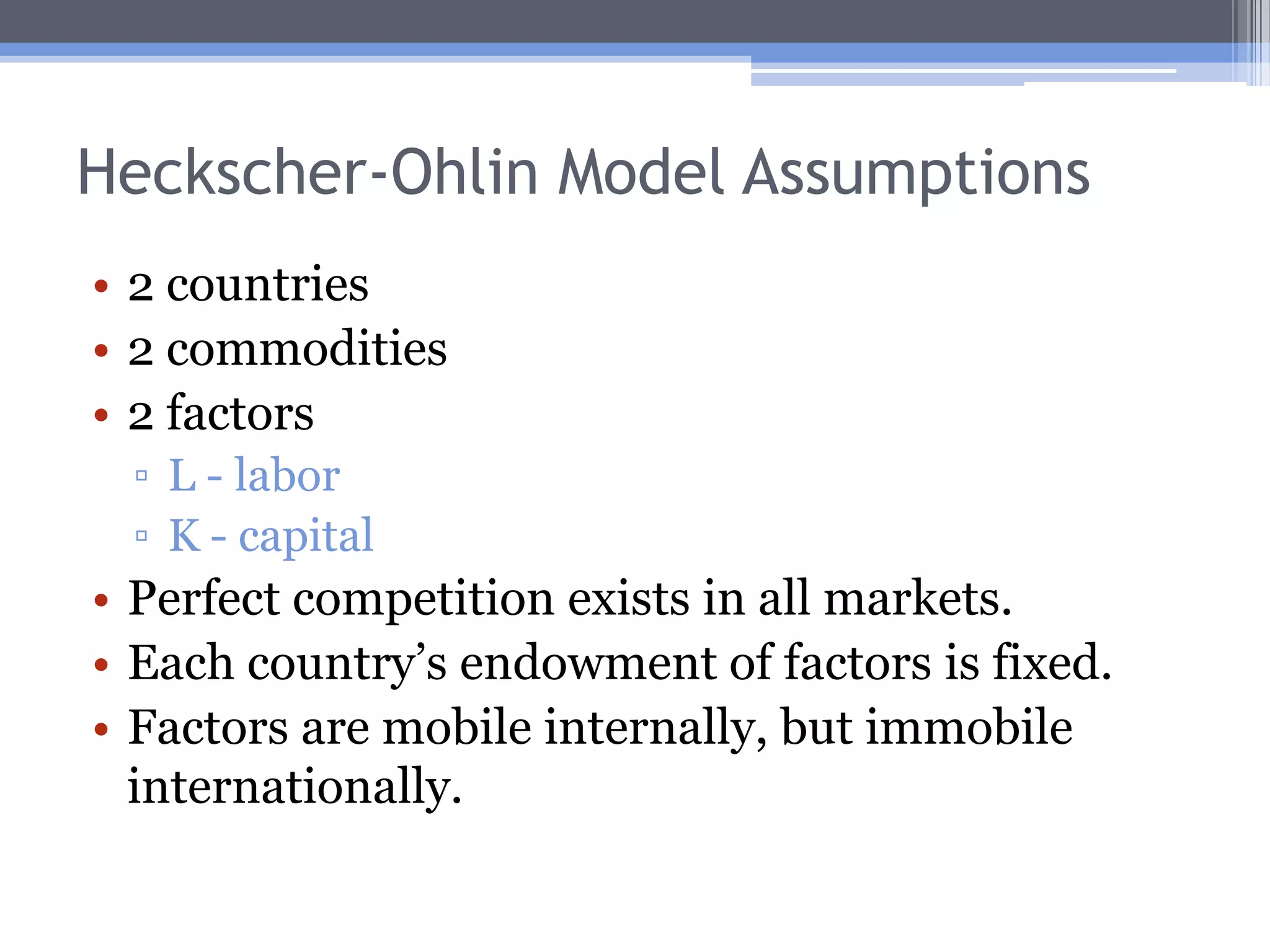
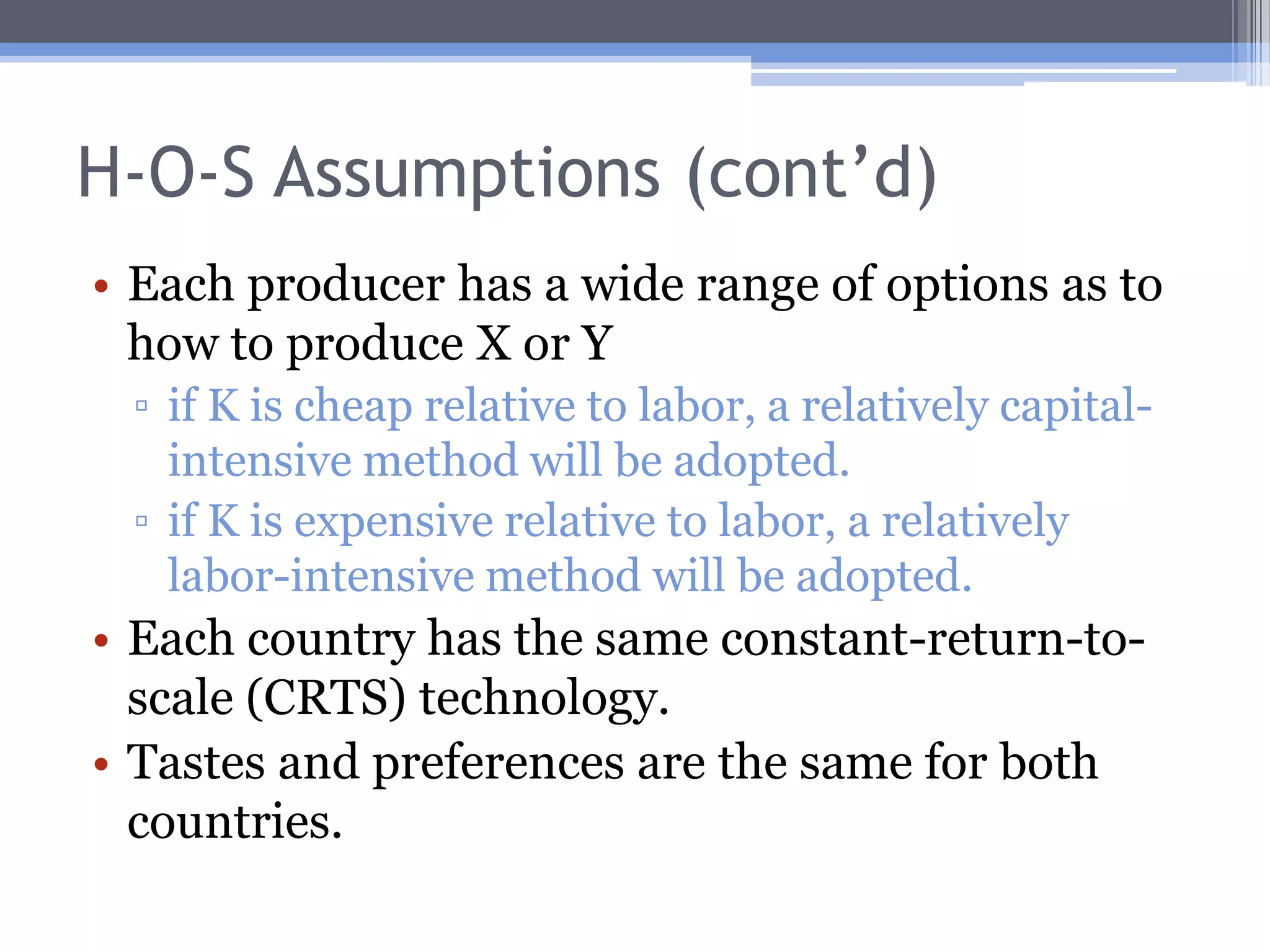
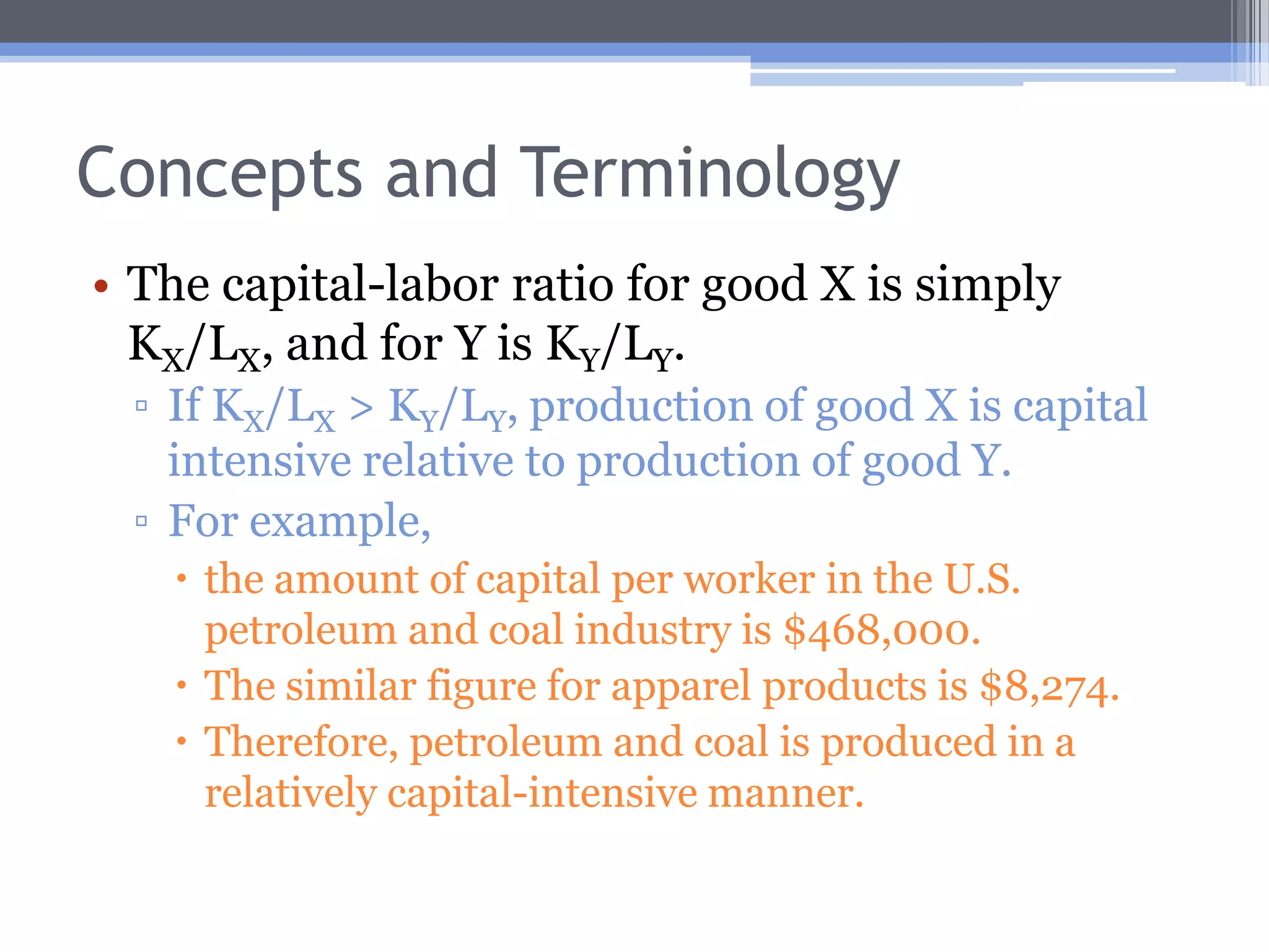
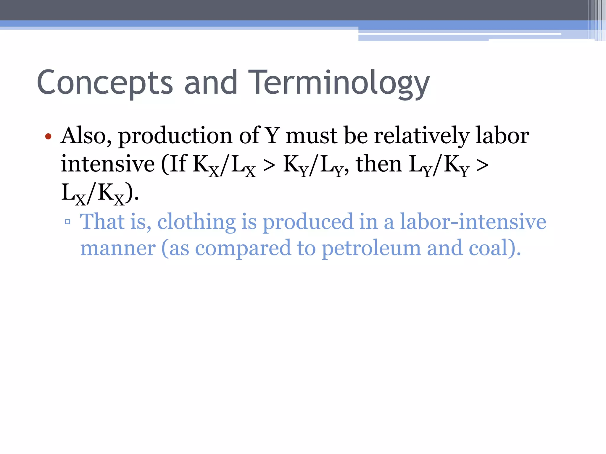
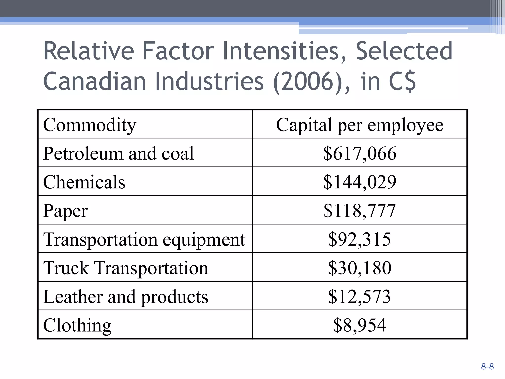
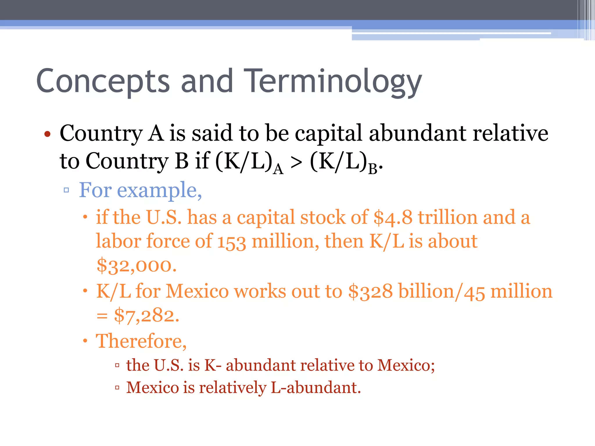
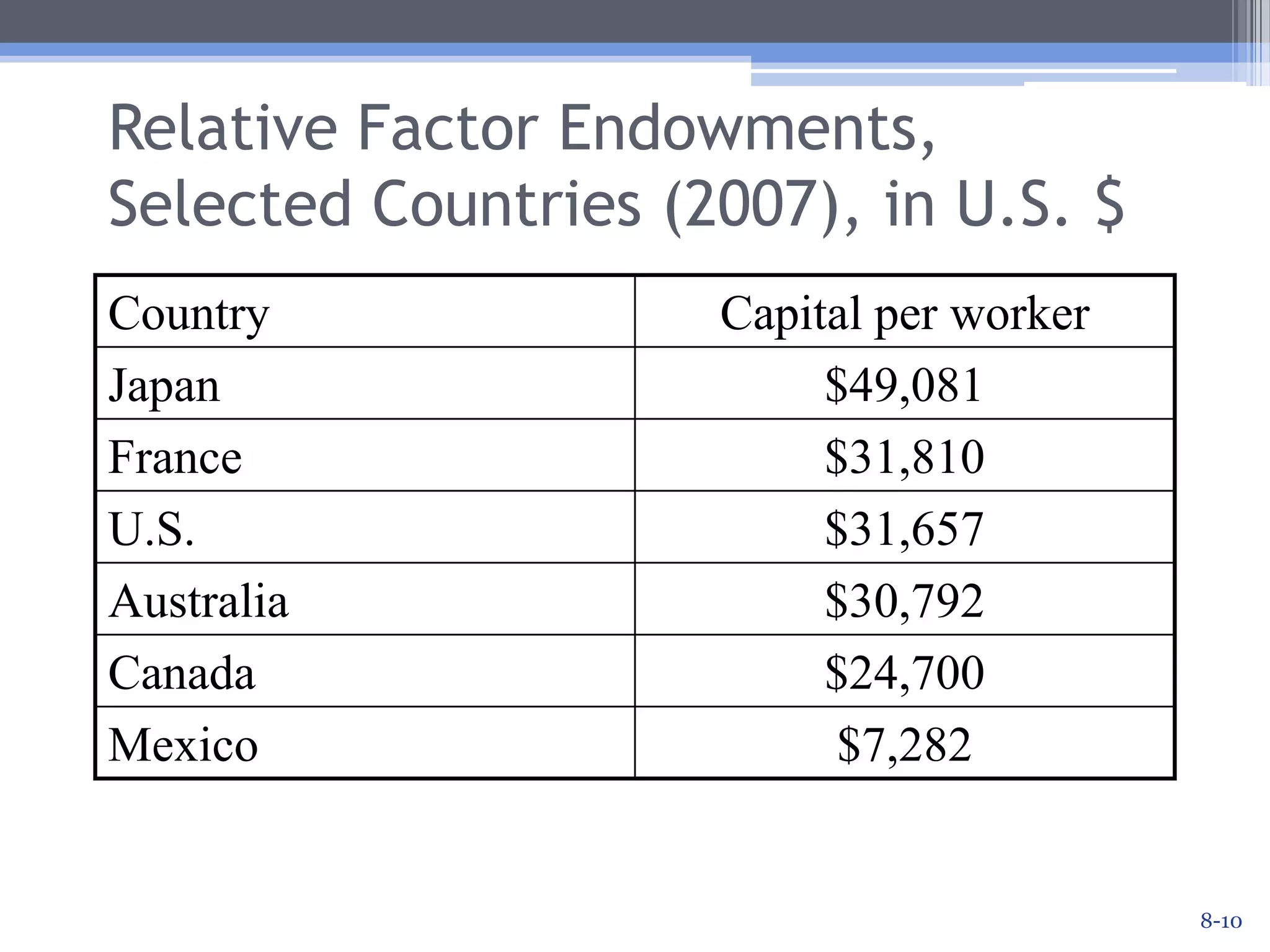
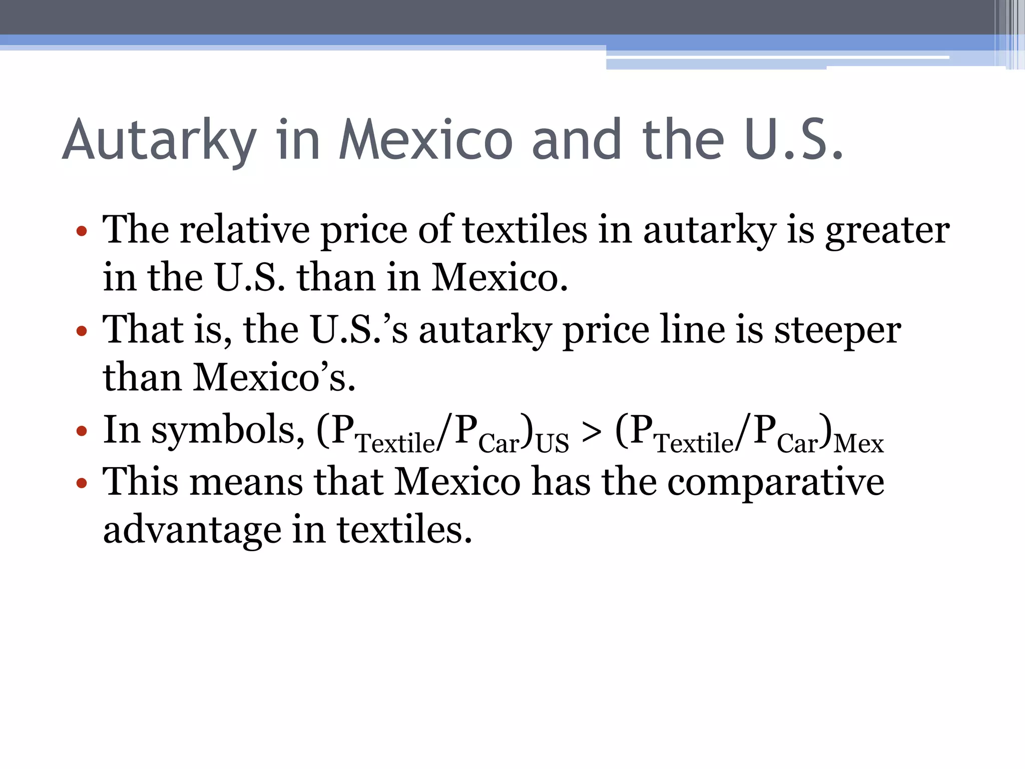
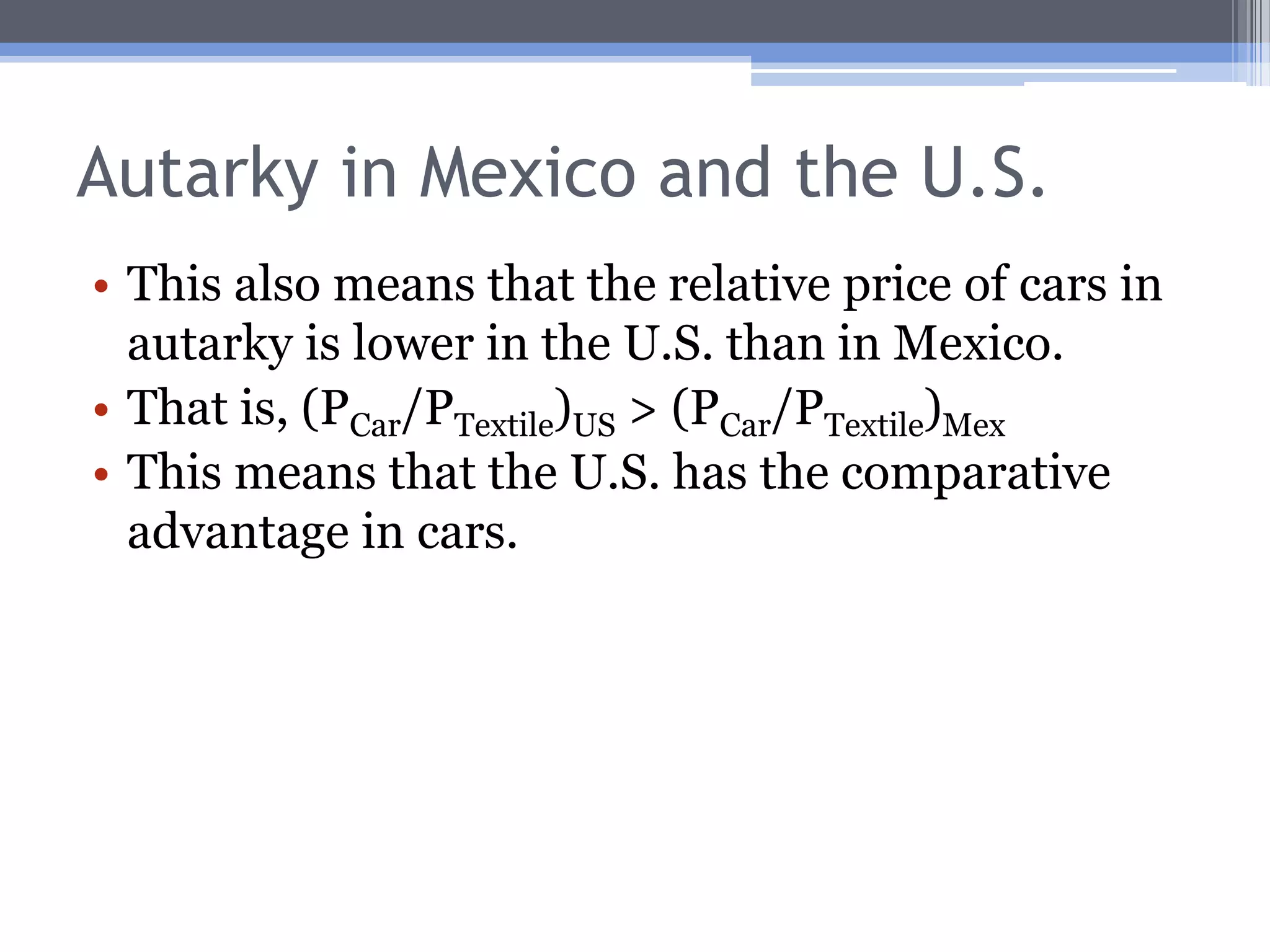
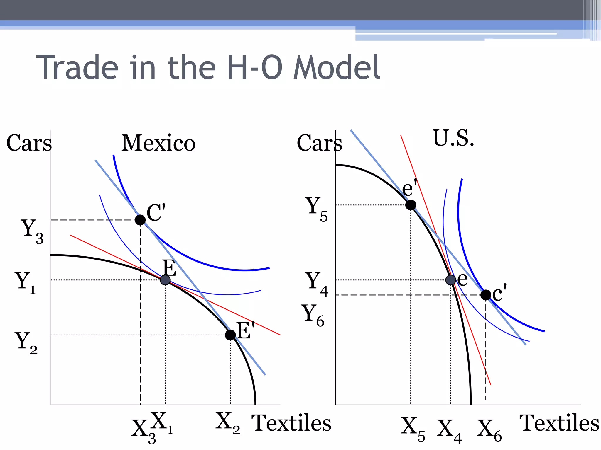
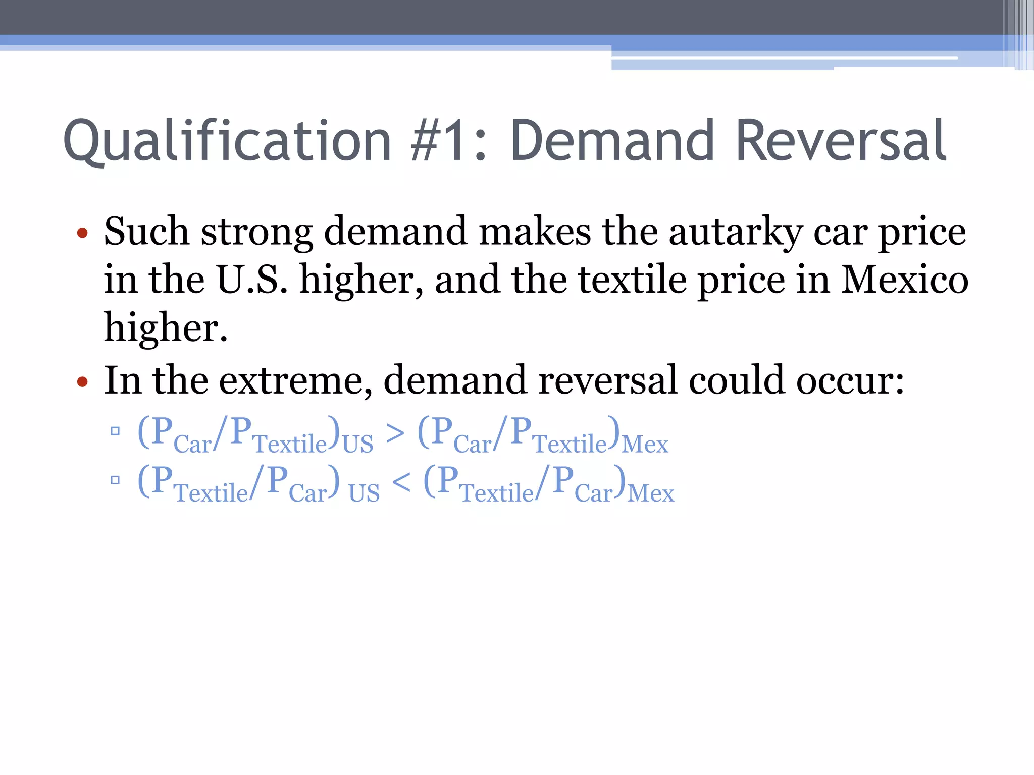
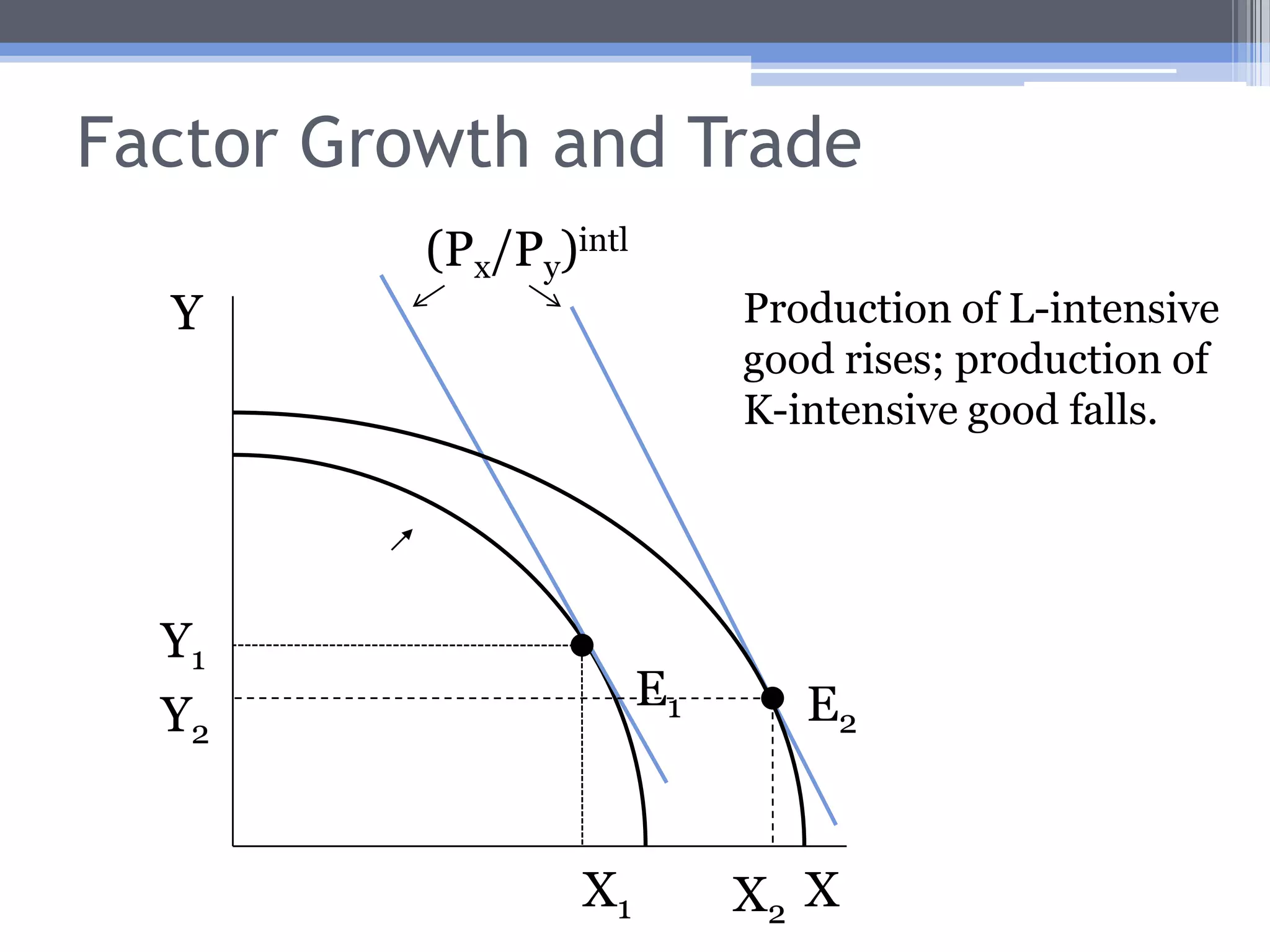
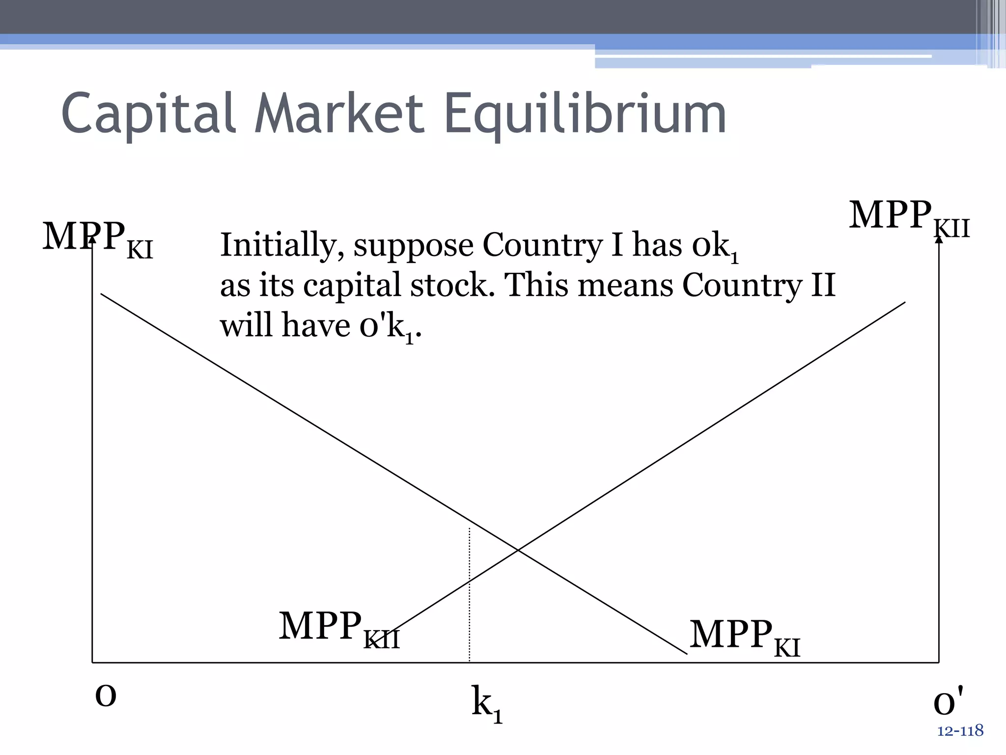
This document provides a summary of the Heckscher-Ohlin model of international trade. It discusses the model's key assumptions, concepts, and implications. The summary is as follows: 1) The Heckscher-Ohlin model examines how differences in countries' factor endowments (e.g. capital vs. labor) lead to comparative advantages and patterns of trade. 2) It assumes two countries, two goods, and two factors of production. If one country is relatively capital-abundant, it will export capital-intensive goods and import labor-intensive goods. 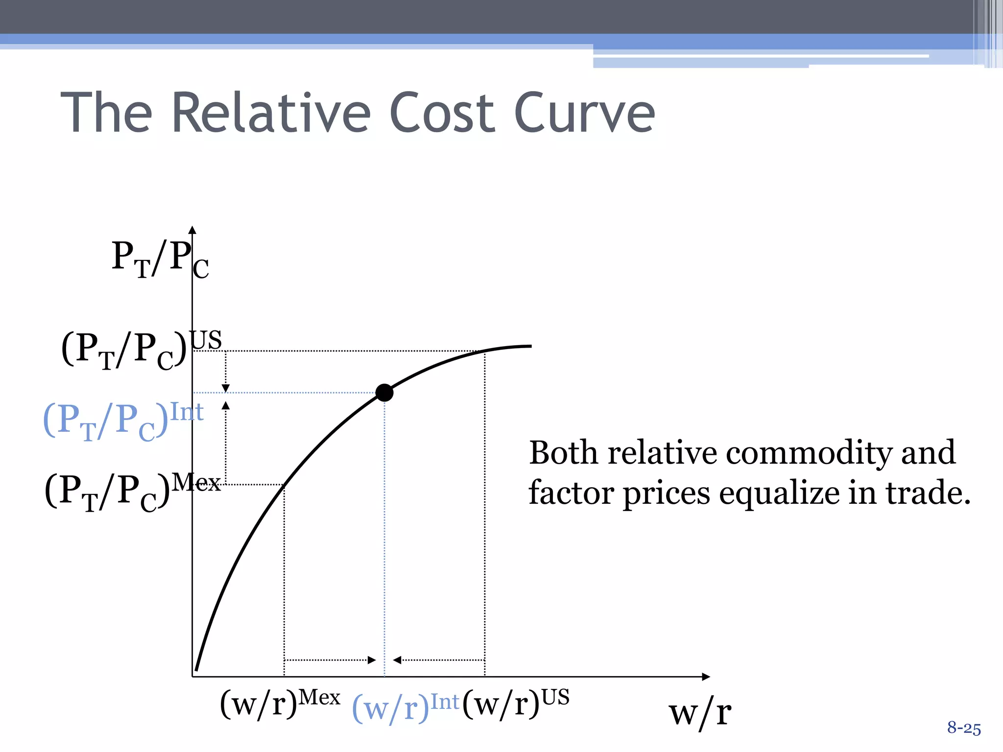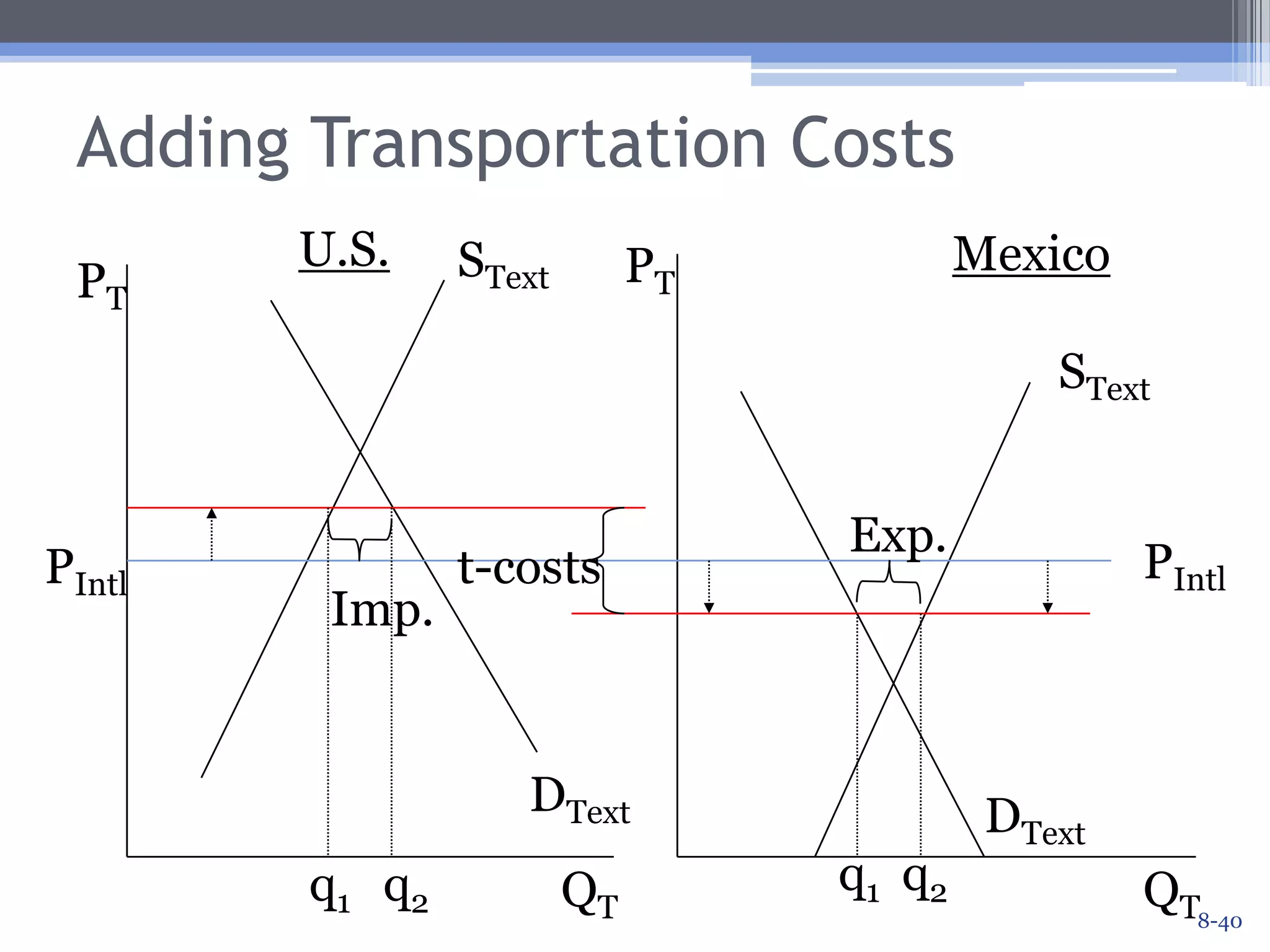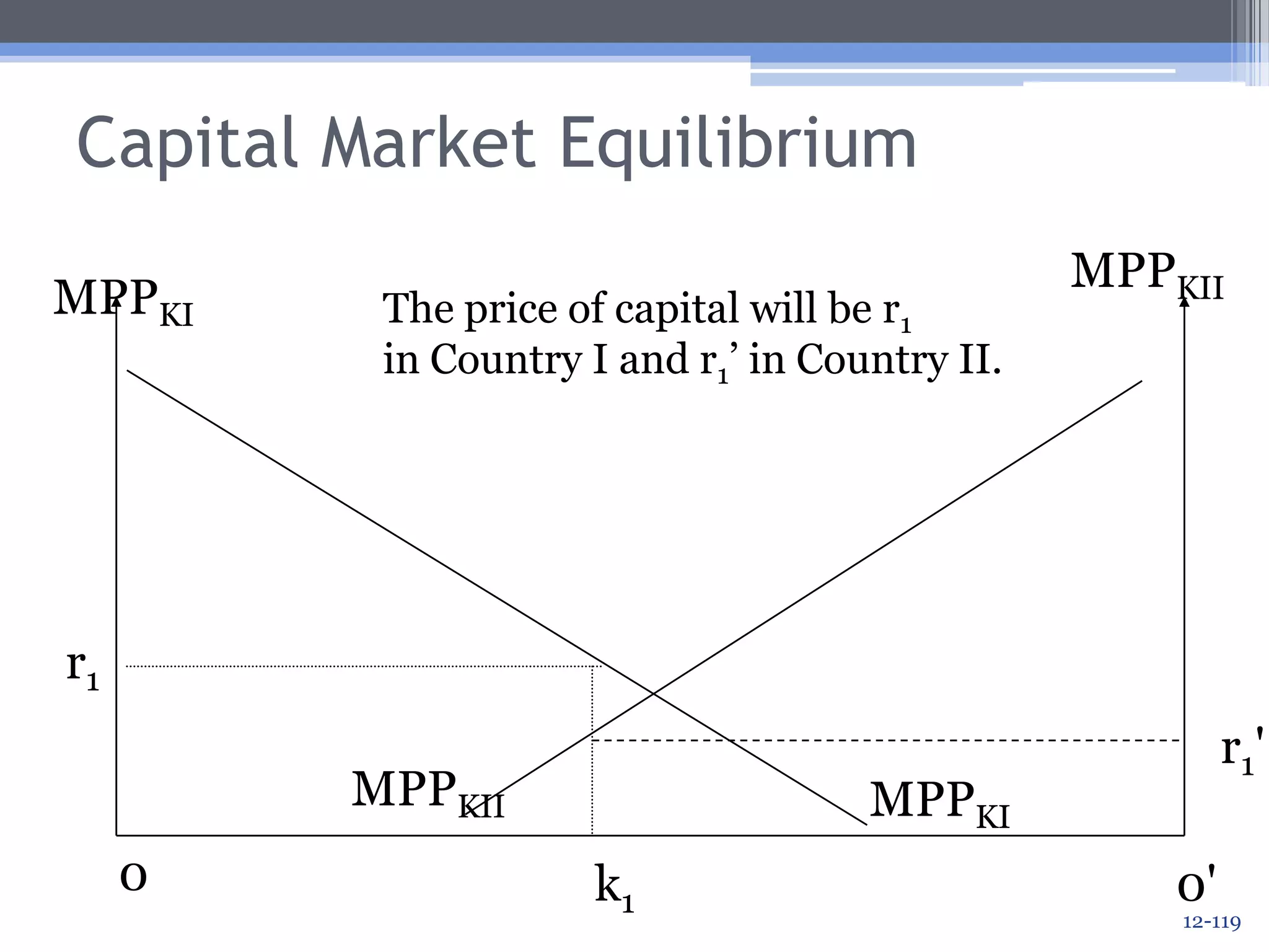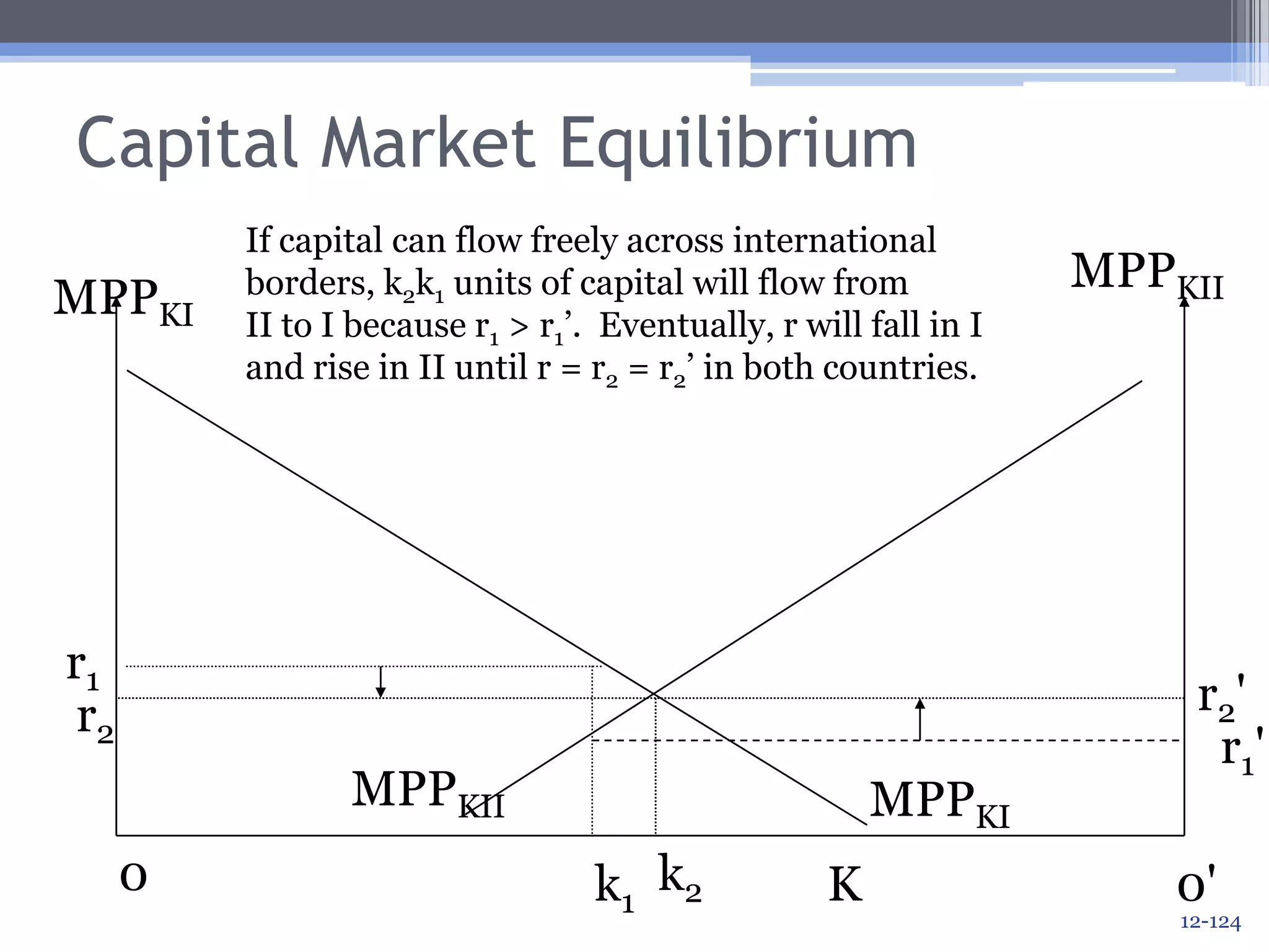3) The model shows that trade equalizes factor prices between countries. This factor price equalization theorem demonstrates how

1. Lecture 5August 9th 2010

2. The Basis for Trade: Factor Endowments and the Heckscher-Ohlin Model

3. Heckscher-Ohlin In GeneralHeckscher, and his student Ohlin, worked in the early part of the 20th century.Paul Samuelson refined their work after WWII.Closer attention is paid in this model to each country’s resource endowment.

4. Heckscher-Ohlin Model Assumptions2 countries2 commodities2 factors L - labor K - capitalPerfect competition exists in all markets.Each country’s endowment of factors is fixed.Factors are mobile internally, but immobile internationally.

5. H-O-S Assumptions (cont’d)Each producer has a wide range of options as to how to produce X or Yif K is cheap relative to labor, a relatively capital-intensive method will be adopted.if K is expensive relative to labor, a relatively labor-intensive method will be adopted.Each country has the same constant-return-to-scale (CRTS) technology.Tastes and preferences are the same for both countries.

6. Concepts and TerminologyThe capital-labor ratio for good X is simply KX/LX, and for Y is KY/LY.If KX/LX > KY/LY, production of good X is capital intensive relative to production of good Y.For example, the amount of capital per worker in the U.S. petroleum and coal industry is $468,000.The similar figure for apparel products is $8,274.Therefore, petroleum and coal is produced in a relatively capital-intensive manner.

7. Concepts and TerminologyAlso, production of Y must be relatively labor intensive (If KX/LX > KY/LY, then LY/KY > LX/KX).That is, clothing is produced in a labor-intensive manner (as compared to petroleum and coal).

8. Relative Factor Intensities, Selected Canadian Industries (2006), in C$8-8

9. Concepts and TerminologyCountry A is said to be capital abundant relative to Country B if (K/L)A > (K/L)B.For example, if the U.S. has a capital stock of $4.8 trillion and a labor force of 153 million, then K/L is about $32,000. K/L for Mexico works out to $328 billion/45 million = $7,282.Therefore, the U.S. is K- abundant relative to Mexico; Mexico is relatively L-abundant.

10. Relative Factor Endowments, Selected Countries (2007), in U.S. $8-10

11. Concepts and TerminologyTo summarize:goods are produced relatively K or L intensively.countries are relatively K or L abundant.

12. Concepts and TerminologyThe factor price of labor (the wage) is “w”The factor price of capital is “r”If labor is relatively expensive, w/r will be a relatively big number.If labor is relatively cheap, w/r will be a relatively small number.

13. More on Factor PricesWhat makes labor relatively expensive?If it is relatively scarce.What makes labor relatively cheap?If it is relatively abundant.So: If (K/L)A is a relatively big number (that is, capital is relatively abundant), w/r will be a relatively big number, reflecting the relative scarcity of L and abundance of K.

14. A Review of Trade in the Neoclassical ModelSuppose the U.S. is capital abundant relative to Mexico.This, of course, means that Mexico is relatively labor abundant.These differences affect the shape of each country’s PPF.Suppose that cars are produced rel. K-intensively, and textiles labor intensively.

15. Autarky in Mexico and the U.S.The relative price of textiles in autarky is greater in the U.S. than in Mexico.That is, the U.S.’s autarky price line is steeper than Mexico’s.In symbols, (PTextile/PCar)US > (PTextile/PCar)MexThis means that Mexico has the comparative advantage in textiles.

16. Autarky in Mexico and the U.S.This also means that the relative price of cars in autarky is lower in the U.S. than in Mexico.That is, (PCar/PTextile)US > (PCar/PTextile)MexThis means that the U.S. has the comparative advantage in cars.

17. Trade in the H-O ModelU.S.MexicoCarsCarse'Y5C'Y3EeY1Y4c'Y6E'Y2X1X2TextilesTextilesX5X6X3X4

18. The ResultThe relatively capital abundant country (U.S.) exports the relatively capital intensive good (cars).The relatively labor abundant country (Mexico) exports the relatively labor intensive good (textiles).

19. The Heckscher-Ohlin TheoremA country will export the commodity that uses relatively intensively the factor that country has in relative abundance.A country will import the commodity that uses relatively intensively the factor that is relatively scarce in that country.

20. The Source of Comparative AdvantageSo it is a country’s relative factor endowment that determines its comparative advantage.This is why the H-O-S model is also called the factor proportions theory.

21. Changes in Relative Commodity Prices : ReviewAs we learned before, (PTextile/PCar)US falls as the U.S. moves to trade. That is, the international relative textile price is lower than the U.S.’s autarky price.(PTextile/PCar)Mex rises as Mexico moves to trade. That is, the international relative textile price is higher than Mexico’s autarky price.

22. Changes in Factor PricesIn autarky, the K-intensive product (cars) is less expensive to produce in the U.S. as compared to Mexico.This is because K is relatively abundant in the U.S., which makes the price of capital relatively low.As trade commences, r will rise since demand for capital will rise.

23. Changes in Factor PricesIn autarky, the L-intensive product (textiles) is more expensive to produce in the U.S. as compared to Mexico.This is because L is relatively scarce in the U.S., which makes the price of labor relatively high.As trade commences, w will fall since demand for labor will fall.

24. Commodity and Factor Prices In Trade: A SummaryIn our example, (PTextile/PCar)US falls as trade commences.(w/r)US also falls.In Mexico, the opposite is happening:(PTextile/PCar)Mex rises.(w/r)Mex also rises.Therefore relative commodity and factor prices move together as trade commences.

25. The Relative Cost CurvePT/PC(PT/PC)US(PT/PC)IntBoth relative commodity and factor prices equalize in trade.(PT/PC)Mex(w/r)Mex(w/r)USw/r(w/r)Int8-25

26. The Factor Price Equalization Theorem (FPE)In equilibrium, with both countries facing the same relative product prices, relative costs will be equalized. This can only happen if relative factor prices are equalized between countries.

27. H-O and the Distribution of IncomeThe H-O theorem, together with the FPE theorem, also tell us about how the incomes of different groups within a country change as trade starts.This provides insight into the politics of free trade.

28. The Stolper-Samuelson Theorem (S-S)As trade commences, the owners of the relatively abundant factor will find their real incomes rising; the owners of the relatively scarce factor will find their real incomes falling.

29. H-O and the Distribution of IncomeAccording to the S-S theorem, if the U.S. is a relatively K-abundant country, who in America should favor free trade?Who in America should favor protectionism?

30. Theoretical Qualifications to H-OSuppose we relax some of the many assumptions. Will the implications of the H-O-S model still be the same?

31. Qualification #1: Demand ReversalSuppose we let demand conditions differ.Suppose domestic demand for the good that uses relatively intensively the relatively abundant factor is very strong in each country.That is, suppose demand for cars is very strong in the U.S., and that demand for textiles is very strong in Mexico.

32. Qualification #1: Demand ReversalSuch strong demand makes the autarky car price in the U.S. higher, and the textile price in Mexico higher.In the extreme, demand reversal could occur: (PCar/PTextile)US > (PCar/PTextile)Mex(PTextile/PCar) US < (PTextile/PCar)Mex

33. Bottom Line on Demand ReversalsIf demand reversals occur, the H-O theorem no longer holds: the K-abundant country is exporting the L-intensive good, and the L-abundant country is exporting the K-intensive good.

34. Qualification #2: Factor Intensity ReversalImplicitly, we’ve assumed that if good X is K-intensive relative to good Y at one factor price ratio, it will be K-intensive at all factor prices.A FIR is when a good is relatively K-intensive at one set of factor prices, but relatively labor intensive at another.

35. Qualification #2: Factor Intensity ReversalFIRs occur when capital and labor can be substituted more easily in the production of one good than another.

36. Factor Intensity Reversal: Implications for TradeSuppose France is K-abundant relative to Germany (that is (K/L)France > (K/L)Germany).This means that (w/r) France > (w/r) Germany.Suppose further that there is a FIR: in France, at (w/r ) France apples are produced relatively K-intensively but in Germany at (w/r ) Germany apples are produced in a relatively L-intensive way.

37. Factor Intensity Reversal: Implications for TradeIf trade begins, according to the H-O theorem the relatively K-abundant country (France) will export the rel. K-intensive good (apples) and the rel. L-abundant country will export the rel. L-intensive good (also apples).H-O theorem breaks down.

38. Qualification #3: Transportation CostsIn the real world, it is costly to transport goods internationally.How do the implications of our model change if we allow for transportation costs?Consider the supply and demand curves for textiles in Mexico and the U.S.

39. Adding Transportation CostsUnless Mexico is the only seller in the world, transportation costs will be borne by both the consumer (the U.S.) and the seller (Mexico).How does this look on the graph?

40. Adding Transportation CostsU.S.MexicoSTextPTPTSTextExp.PIntlPIntlt-costsImp.DTextDTextq1q2q1q2QTQT8-40

41. Adding Transportation Costs: the Bottom LineIn general, the H-O theorem will still hold.The FPE theorem breaks down, since factor prices only equalize if the commodity prices do.Therefore, in the presence of transportation costs, factor prices have a tendency to move towards each other, but we should not expect equalization.

42. Relaxing Other AssumptionsOne can relax many other assumptions and examine how the implications of the model change:perfect competitionCRTSidentical production technologieslack of policy obstaclesfactors being perfectly transferable

43. Post–Heckscher-Ohlin Theories of Trade and Intra-Industry Trade

44. Posner’s Imitation Lag HypothesisIn Posner’s model, there may be a delay in the diffusion of technology between countries.If a new product is invented in country I, there are two sorts of lags that delay the production the good in country II: imitation lag, anddemand lag.During these lags the inventing country will export.

45. The Product Cycle ModelHow might comparative advantage change over time? H-O is a static model, and therefore offers little info on this.The Product Cycle model (Vernon, 1966) follows a product from its invention through its “old age.”How does it work?

46. The Product Cycle Model: The New Product Phase A new product is invented in the developed world.Typically, the new product will becapital-intensive and labor-saving.aimed at high-income consumers.All demand is located in the inventing country.

47. The Product Cycle Model: The New Product PhaseProduction is located in the inventing country.Technological uncertainties make mass production unfeasible.No trade occurs during this phase.

48. The Product Cycle Prodn, consnInventing country consumption Inventing country productiontimet0t1New product phase

49. The Product Cycle Model: The Maturing Product PhaseThe product is increasingly standardized.Consumers are increasingly aware of the product.Mass production becomes possible, and economies of scale are realized.Price steadily drops.Demand in other developed countries picks up, so inventing country producers export more and more.

50. The Product Cycle Model: The Maturing Product PhaseLater in the maturing product phase, other developed countries begin to produce the product.Lower transportation costs may give these new entrants an edge in the emerging markets.Increasingly, output in the inventing country is displaced.

51. The Product Cycle Prodn, consnInventing country consumptionexportsInventing country production timet0t1t2New product phaseMaturing product phase

52. The Product Cycle Model: The Standardized Product PhaseGlobal demand has grown.Production techniques are well-known and standard.Competition becomes ever fiercer.As a result, production shifts mainly to developing countries.Product differentiation may occur, with the inventing country left producing only fancier versions.The inventing country becomes a net importer.

53. The Product Cycle Prodn, consnInventing country consumptionimportsexports Inventing country productiontimet0t1t2New product phaseMaturing product phaseStandardized product phase10-53

54. The Product Cycle TheoryVernon’s Product Cycle theory tells us that comparative advantage is fleeting: we need to perpetually invent new products.

55. Vertical SpecializationDifferent stages of production process may occur in different countries.If different parts of the production process vary in terms of capital or labor intensity, the production process may be spread over multiple countries.

56. Firm-Focused TheoriesStage theory: owners and managers learn over time; this implies exporting firms tend to be larger and run by more experienced managers.Resource-exchange theory: firms internationalize because they cannot generate all resources domestically.Network theory: networking can compensate for any lack of experience or expertise.

57. The Linder TheoryIn the H-O model, the pattern of trade is determined by relative resource endowments.A model by Linder (1961) focuses mainly on the demand side.Basic idea is that a country produces stuff to satisfy domestic demand; these goods will be likely exports (and imports, too).

58. The Linder Theory: An ExampleSuppose Country I’s income pattern is such that it produces goods A, B, C, D and E.Let Country I have a relatively low per capita income level.Suppose these goods are in ascending order of sophistication:A and B are fairly simple.C, D, and E are slightly more sophisticated.

59. The Linder Theory: An ExampleSuppose Country II has a higher level of per capita income.It therefore produces goods C, D, and E (just like Country I), but also F and G.F and G are even more sophisticated.

60. The Linder Theory: An ExampleSuppose Country III has an even higher level of per capita income.It therefore produces good E (just like Country I), F and G (just like country II), but also H and J.H and J are even more sophisticated.Let’s look at a diagram of these countries:

61. The Linder Theory: An ExampleWhat products will I and II trade? IABCDEC, D, and E.IIGCDEFIIIGEFHJ10-61

62. The Linder Theory: An ExampleWhat products will II and III trade? IABCDEE, F, and G.IIGCDEFIIIGEFHJ10-62

63. The Linder Theory: An ExampleWhat products will I and III trade? IABCDEE only.IIGCDEFIIIGEFHJ10-63

64. The Linder TheorySo trade will involve goods for which there is overlapping demand.Implication: trade should be most intense between countries with similar levels of per capita income.

65. The Linder TheoryThis theory would explain two things that H-O cannot:why most trade is between the industrialized countries, which all have (presumably) very similar resource endowments.why a country might import and export the same product (intra-industry trade).

66. The Linder TheoryThe theory has been subjected to a barrage of tests.Sailors, et al. (1973), Thursby and Thursby (1987), and McPherson, Redfearn and Tieslau (2000) and others found evidence to support the Linder theory.Hoftyzer (1984), Kennedy and McHugh (1983) and others found evidence against the theory.

67. The Krugman ModelIncorporates economies of scale and monopolistic competition.Consider a graph:The price of the good relative to the wage (P/W) is on the vertical axis.Per capita consumption (c) is on the horizontal axis.

68. The Krugman ModelTwo functions are on the graph:The PP curve slopes upward, since P/W increases as c increases.The ZZ curve has a negative slope: as c increases, average cost decreases (due to economies of scale). To maintain the zero-profit condition in monopolistically competitive firms, price must be reduced.

69. The Krugman ModelPoint E is the initial equilibrium, with thefirm maximizing itsprofit, and earning zero economic profit.P/WPZE(P/W)1ZPc1c

70. The Krugman ModelSuppose this firm exists in country 1.Let country 2 be identical to country 1 on both the demand and the supply sides of the economy.Traditional trade theory posits that these countries would not trade.However, because trade effectively increases the market size in each country, economies of scale are realized in the Krugman model.Trade effectively shifts the ZZ curve to the left.

71. The Krugman ModelPoint E΄ is the newequilibrium; per capita consumption and P/W have both decreased as a result of trade.P/WPZZ΄E(P/W)1E΄(P/W)2ZPZ΄c1c2c

72. The Krugman Model: The Bottom LineAlthough trade causes per capita consumption (c) to fall, total consumption of the firm’s output has risen.P/W has decreased because of trade; this also means that its reciprocal (W/P) rises.This suggests that trade causes the real wage of workers to rise.Even owners of the relatively scarce factor see a rise in real wages, suggesting that the negative income distribution effects of trade may not occur.

73. Other Trade ModelsReciprocal dumping model (Brander and Krugman, 1983)Because of imperfect competition, intra-industry trade occurs in this model.Welfare may increase due to increased competition, but may decrease due to waste involved with transporting identical products internationally; the overall welfare effect is unclear.The gravity modelThe focus is on explaining trade volume.These models illuminate the underlying causes of trade.

74. Intra-Industry TradeExamples:Japan imports and exports computers.The Netherlands imports and exports beer.The U.S. imports and exports broccoli.H-O-S is useless in explaining this - there’s no way a country could export and import the same good.

75. Intra-Industry Trade: Possible ExplanationsProduct differentiationTransportation costsDynamic economies of scaleDegree of product aggegationDiffering national income distributionsDiffering factor endowments and product variety

76. How Common is Intra-Industry Trade?A recent study by Brülhart attempts to measure IIT in several countries, using an index:an index value of 0 implies no IIT is taking place.an index value of 1 implies that a country’s exports in one product category exactly equal its imports.

77. Intra-Industry Trade: Evidence from Brülhart (2009)

78. Economic Growth and International Trade

79. IntroductionHow does economic growth in China affect other countries?Has China’s growth come at the expense of other countries?

80. The Trade Effects of GrowthAs real income rises, producers are affected: how should they alter production in response?consumers are also affected: how should they spend the additional income?

81. Trade Effects of Production GrowthIf a country experiences growth its PPF will shift outwards.The producers in that country will now have the chance to select a production point on the new PPF.Suppose a country exports good X and imports good Y.

82. Trade Effects of Production GrowthYIIIIVIIIAX

83. Trade Effects of Production GrowthNew production points in region II of the new PPF involve production of more of the export good (Y) and less of the import good (X).This is ultra-protrade production growth.This means the growth has a strong positive effect on the country’s desire to trade.

84. Trade Effects of Production GrowthNew production points in region I of the new PPF involve production of more of the both goods, but proportionately more of the export good (X).This is protrade production growth.This growth will have a positive effect on the country’s desire to trade.

85. Trade Effects of Production GrowthNew production points in region IV of the new PPF involve production of more of the import good (Y) and less of the export good (X).This is ultra-antitrade production growth.This means the growth has a strong negative effect on the country’s desire to trade.

86. Trade Effects of Production GrowthNew production points in region III of the new PPF involve production of more of the both goods, but proportionately more of the import good (Y).This is antitrade production growth.This growth will have a negative effect on the country’s desire to trade.

87. Trade Effects of Consumption GrowthIf a country experiences growth, the consumers in that country will now have the chance to select a new consumption point.Let us continue to suppose a country exports good X and imports good Y.To focus on consumption, we’ll look only at the consumption possibilities frontier (CPF).

88. Trade Effects of Consumption GrowthIIIIVYIIIBCPFX

89. Trade Effects of Consumption GrowthNew consumption points in region II of the new CPF involve consumption of more of the export good (Y) and less of the import good (X).This is ultra-antitrade consumption effect.This means the growth has a strong negative effect on the country’s desire to trade.

90. Trade Effects of Consumption GrowthNew consumption points in region I of the new CPF involve consumption of more of the both goods, but proportionately more of the export good (X).This is antitrade consumption effect.This growth will have a negative effect on the country’s desire to trade.

91. Trade Effects of Consumption GrowthNew consumption points in region IV of the new CPF involve consumption of more of the import good (Y) and less of the export good (X).This is ultra-protrade consumption effect.This means the growth has a strong positive effect on the country’s desire to trade.

92. Trade Effects of Consumption GrowthNew consumption points in region III of the new PPF involve consumption of more of the both goods, but proportionately more of the import good (Y).This is a protrade consumption effect.This growth will have a positive effect on the country’s desire to trade.

93. Production and Consumption Effects CombinedTo summarize the combined production and consumption effects of growth, we look at the income elasticity of demand for imports (YEM).YEM is the percentage change in imports divided by the percentage change in national income.

94. Production and Consumption Effects CombinedYEM = 1: neutral effect0 < YEM < 1: antitrade effectYEM < 0: ultra-antitrade effectYEM > 1: protrade or ultra-protrade effect

95. Sources of GrowthTechnological changeFactor-neutral: results in same relative amounts of K and L are used.Labor-saving: results in increases in relative amount of capital used.Capital-saving: results in increases in relative amount of labor used.

96. Technological Change: Commodity-neutralYX

97. Technological Change: Commodity-specificYYXX11-97

98. Sources of GrowthFactor GrowthFactor-neutral: K and L grow at the same rate.Growth in KGrowth in L

99. Factor Growth: Factor-neutralYX

100. Factor Growth: Factor-specificGrowth of factor in which good Y production is intensive.Growth of factor in which good X production is intensive.YYXX11-100

101. Factor Growth and Trade: Small Country CaseSuppose good X is relatively labor-intensive, and Y is capital intensive.Economic growth shifts the PPF disproportionately along the X-axis.Since country is small international prices don’t change.

102. Factor Growth and Trade(Px/Py)intlYProduction of L-intensive good rises; production of K-intensive good falls.Y1E1E2Y2XX1X2

103. Factor Growth and Trade: the Rybczynski TheoremGrowth in one factor of production leads to an absolute expansion of output of the product using that factor intensively and an absolute contraction of output of the product using the other factor intensively.

104. Factor Growth and Trade: the Rybczynski TheoremIf the abundant factor grows, there will be an ultra-protrade production effect. If the scarce factor grows, there will be an ultra-antitrade production effect.If the consumption effect is protrade, growth in abundant factor will increase trade overall; growth in scarce factor causes the opposite.

105. Growth and Trade: Welfare EffectsGrowth in K or technological improvements will generally increase welfare, since both increase real per capita income and allow a country to reach a higher indifference curve.Growth in L may or may not increase welfare.

106. Factor Growth and Trade: Large Country CaseSuppose a large country experiences growth in its abundant factor.There will be an ulra-protrade production effect.Assuming a neutral consumption effect, the growth will cause an increase in demand for imports and an increase in the supply of exports.The increased willingness to trade leads to a deterioration in the country’s terms of trade.

107. Large Country Case(Px/Py)0YGrowth causes a decline in the TOT to (Px/Py)1. Growthincreases welfare, but not as much as in the small country case. C1C2C0E2E0E1(Px/Py)1X

108. Growth and Trade: Immiserizing GrowthIt is possible that the deterioration in the terms of trade will be large enough that a country with growth finds itself on a lower indifference curve.This phenomenon was dubbed “immiserizing growth” by Jagdish Bhagwati.

109. Immiserizing Growth(Px/Py)0Growth causes a large enough decline in that welfare is reduced.YC0C1C2E2(Px/Py)1E0E1X

110. Growth and the Terms of Trade: Developing CountriesDeveloping countries may experience declining terms of trade as they grow; this suggests a strategy of export product diversification.Income elasticities of demand for minerals and food products tend to be low; those for manufactured goods tend to be higher.Prices of non-petroleum primary products have generally declined over time.

111. International Factor Movement

112. Factors of Production: Capital Types of capital foreign investmentForeign Direct Investment (FDI) Foreign Portfolio Investment (FPI)FDI: Can involve individuals but the bulk is done by firms.known as: Multinational corporations (MNCs)Multinational Enterprise (MNE)Transnational Corporation (TNC)Transnational Enterprise (TNE)

113. Global FDI FlowsIn 2007, the accumulated stock of global FDI was over $15 trillion.This stock grows rapidly each year – 22% in 2007 alone.

114. U.S. FDI Abroad by Industry, 2007

115. U.S. FDI Abroad by Region or Country, 2007

116. World’s Largest Corporations, 2008 (billions of $)12-116

117. Reasons for International Movement of CapitalTo access growing markets.To secure access to raw materials.To avoid tariffs and NTBs.To take advantage of low wages.Defensive purposes to prevent loss of market share.Risk diversification.MNC efficiency over local suppliers.

118. Capital Market EquilibriumMPPKIIMPPKIInitially, suppose Country I has 0k1as its capital stock. This means Country II will have 0'k1.MPPKIIMPPKI0k10'12-118

119. Capital Market EquilibriumMPPKIIMPPKIThe price of capital will be r1in Country I and r1’ in Country II.r1r1'MPPKIIMPPKI0k10'12-119

120. Capital Market EquilibriumMPPKIIMPPKIOutput in Country Ir1r1'MPPKIIMPPKI0k10'12-120

121. Capital Market EquilibriumMPPKIIMPPKIPayment to LaborPayment to Capitalr1r1'MPPKIIMPPKI0k10'12-121

122. Capital Market EquilibriumMPPKIIMPPKIOutput in Country IIr1r1'MPPKIIMPPKI0k10'12-122

123. Capital Market EquilibriumMPPKIIMPPKIPayment to LaborPayment to Capitalr1r1'MPPKIIMPPKI0k10'12-123

124. Capital Market EquilibriumIf capital can flow freely across international borders, k2k1 units of capital will flow from II to I because r1 > r1’. Eventually, r will fall in Iand rise in II until r = r2 = r2’ in both countries.MPPKIIMPPKIr1r2'r2r1'MPPKIIMPPKI0k2Kk10'12-124

125. Capital Market EquilibriumMPPKIIMPPKIWhat happens to output in Country I? It rises due to the capital inflow.Increase in outputr1r2'r2r1'MPPKIIMPPKI0k2Kk10'12-125

126. Capital Market EquilibriumMPPKIIMPPKIWhat happens to output in Country II? It falls because of the loss of capital.r1r2'r2r1'MPPKIIMPPKI0k2Kk10'12-126

127. Capital Market EquilibriumMPPKIIMPPKIWhat happens to output in Country II? It falls because of the loss of capital.Output after capital outflowLoss in outputr1r2'r2r1'MPPKIIMPPKI0k2Kk10'12-127

128. Capital Market EquilibriumMPPKIIMPPKIOverall, world output rises.r1r2'r2r1'MPPKIIMPPKI0k2Kk10'12-128

129. Economic Effects of International Capital Flows On IncomesOutput rises in country I (the country to which the capital flows), BUT:Returns fall for capitalists, since their rate of return decreases.Returns rise for laborers.Capitalists are hurt; labor benefits.Therefore, per capita income rises in Country I.

130. Economic Effects of Int’l Capital Flows On IncomesMPPKIIMPPKILoss by capitalists in Country Ir1r2'r2r1'MPPKIIMPPKI0k2Kk10'12-130

131. Economic Effects of Int’l Capital Flows On IncomesMPPKIIMPPKIGain by laborers in Country Ir1r2'r2r1'MPPKIIMPPKI0k2Kk10'12-131

132. Economic Effects of Int’l Capital Flows On IncomesMPPKIIMPPKINet income gain in Country Ir1r2'r2r1'MPPKIIMPPKI0k2Kk10'12-132

133. Economic Effects of Int’l Capital Flows On IncomesOutput falls in country II (the country from which the capital flows), BUT:Returns rise for capitalists, since their rate of return increases.Returns for laborers fall.Capitalists are better off; labor is worse off.Because overall incomes rise, per capita income rises.

134. Economic Effects of Int’l Capital Flows On IncomesMPPKIIMPPKIIncome gain by capitalists in Country IIr1r2'r2r1'MPPKIIMPPKI0k2Kk10'12-134

135. Economic Effects of Int’l Capital Flows On IncomesMPPKIIMPPKILost labor incomer1r2'r2r1'MPPKIIMPPKI0k2Kk10'12-135

136. Economic Effects of Int’l Capital Flows On IncomesMPPKIIMPPKIOverall gain in income in Country IIr1r2'r2r1'MPPKIIMPPKI0k2Kk10'12-136

137. International Capital Flows: A SummaryBoth countries’ incomes rise as a result of capital flows.World output rises.Capitalists in inflow country (Country I) and Laborers in outflow country (Country II).Capitalists in outflow country (Country II) and Laborers in inflow country (Country I) are better off.

138. Potential Benefits of FDI to Host CountryIncreased outputIncreased wagesIncreased employmentIncreased exportsIncreased tax revenuesRealization of economies of scaleImport of technical and managerial skillsWeakening power of domestic monopoly

139. Potential Costs of FDI to Host CountryAdverse impact in the country’s commodity terms of tradeTransfer pricingDecrease in domestic savingsDecrease in domestic investmentInstability in the balance of paymentsLoss of control over domestic policy

140. Potential Costs of FDI to Host Country (cont’d)Increase in UnemploymentEstablishment of Local MonopolyInadequate attention to the development of local education and skills Loss of natural resources

141. Why Migrate?Simply put, migration occurs when the expected costs of migrating are less than the expected benefits.

142. Economic Effects of Labor MigrationGDP in Country I is given by the shaded area:MPPLIIWIIMPPLIWIIncome of capitalistsIncome of laborerswIIwIIwIwIMPPLIIMPPLI0'L2012-142

143. Economic Effects of Labor MigrationGDP in Country II is given by the shaded area:MPPLIIWIIMPPLIWIIncome of capitalistsIncome of laborerswIIwIIwIwIMPPLIMPPLII0'L2012-143

144. Economic Effects of Labor MigrationIf migration is possible, 0L1 workers will work in Country I and 0'L1 in Country II. The wage will be the same: Weq.MPPLIIWIIMPPLIWIwIIwIIweqweqwIwIMPPLIIMPPLI0'L20L112-144

145. Economic Effects of Labor MigrationWhat happens to Country I? GDP fallsbecause of out-migration:MPPLIIWIIMPPLIWILost GDPwIIwIIweqweqwIwIMPPLIIMPPLI0'L20L112-145

146. Economic Effects of Labor MigrationGDP falls in country I (the country from which the migrants come), BUT:Wages rise for remaining workers.It can be shown that the decrease in the Country I labor force is greater than the decrease in GDP, so per capita income rises.Capitalists are hurt; labor benefits.

147. Economic Effects of Labor MigrationWhat happens to Country II? GDP risesbecause of in-migration:MPPLIIWIIMPPLIWIIncrease in GDPIIwIIwIIweqweqwIwIMPPLIMPPLII0'L2012-147

148. Economic Effects of Labor MigrationGDP rises in country II (the country to which migrants go), BUT:Wages fall.It can be shown that the increase in the Country II labor force is greater than the increase in GDP, so per capita income falls.Labor is worse off; capitalists are better off.

149. Economic Effects of Labor MigrationCountry I’s loss in GDP is smaller than Country II’s gain, so world GDP rises.MPPLIIWIIMPPLIWIIncrease in GDPIIwIIwIIweqweqwIwIMPPLIMPPLII0'L2012-149

150. Economic Effects of Labor MigrationCountry I’s loss in GDP is smaller than Country II’s gain, so world GDP rises.MPPLIIWIIMPPLIWIDecrease in GDPIwIIwIIweqweqwIwIMPPLIMPPLII0'L2012-150

151. Economic Effects of Labor MigrationCountry I’s loss in GDP is smaller than Country II’s gain, so world GDP rises.MPPLIIWIIMPPLIWIIncrease in Total GDPwIIwIIweqweqwIwIMPPLIMPPLII0'L2012-151

152. International Migration: Other ConsiderationsMigrants now in Country II may send remittances back to Country ISo I’s per capita income rises by even more, andII’s per capita income falls by even more.If the migrants are “guest workers” and they can be paid a lower wage, it may be possible for capitalists in Country II to be better off without domestic labor being worse off.

153. International Migration: Other ConsiderationsIf the immigrants are low-skill workers, the host country may experience rising social costs.If the immigrants are high-skill workers, the host country may benefit, and the migrants’ home countries may suffer. This is called the “brain drain.”