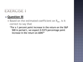
Solution Manual Advanced Accounting by Baker 9e Chapter 16Saskia Ahmad
Solution Manual, Advanced Accounting, Thomas E. King, Cynthia Jeffrey, Richard E. Baker, Valdean C. Lembke, Theodore Christensen, David Cottrell, Richard Baker, Advanced Financial Accounting, Advanced Financial Accounting by Baker Chapter 18, Advanced Financial Accounting by Baker Chapter 18 9th Edition, 9th Edition,
Solution Manual Advanced Financial Accounting by Baker 9th Edition Chapter 16Saskia Ahmad
Solution Manual, Advanced Accounting, Thomas E. King, Cynthia Jeffrey, Richard E. Baker, Valdean C. Lembke, Theodore Christensen, David Cottrell, Richard Baker, Advanced Financial Accounting, Advanced Financial Accounting by Baker Chapter 18, Advanced Financial Accounting by Baker Chapter 18 9th Edition, 9th Edition,
Solution Manual Advanced Accounting Chapter 15 9th Edition by BakerSaskia Ahmad
Solution Manual, Advanced Accounting, Thomas E. King, Cynthia Jeffrey, Richard E. Baker, Valdean C. Lembke, Theodore Christensen, David Cottrell, Richard Baker, Advanced Financial Accounting, Advanced Financial Accounting by Baker Chapter 18, Advanced Financial Accounting by Baker Chapter 18 9th Edition, 9th Edition,
All companies are the topic to the bankruptcy risks. If we look at the definition, a bankruptcy risk is
the business’ disability to deal with payable responsibilities. In the recent past, as a consequence of the
dynamization of the financial and economic action of different firms, it has become essential to obtain precise
information about bankruptcy. In order to summarize this analysis, I use a binary logistic regression because it
is important to verify if some financial
BA 3010 Assignment #1During this course, you will be graded on.docxwilcockiris
BA 3010 Assignment #1
During this course, you will be graded on three dimensions:
1. your ability to identify the correct analytical tool to use,
2. your ability to execute the analysis you have selected,
3. your ability to interpret the results of your analysis
To that end, the assignments will try to reinforce those particular skills by directly targeting these dimensions.
All of your work should be done in an Excel spreadsheet, including your text responses. Do not send in a Word document. You should submit your assignment via the submission process in Blackboard.
Identify
Q1) Open up the file Assignment 1 and examine the data set on the worksheet Q1. This is a data set of 500 Bakersfield households that were recently surveyed. A definition for each variable (unless self-explanatory) can be found in the comments section (place your cursor over any cell with a little red triangle – a comment box will pop up). Our objective is to learn about the financial state of all Bakersfield households. Answer the following (a text box for your answers is provided to the right of the data):
a) Is this cross-sectional data or time-series data?
b) Is this a population or a sample?
c) Ignoring the variable Household, which is just an identifier variable (household #1, household #2, etc.), identify the variable type and sub-type for each variable.
d) If you wished to examine the distribution of the variable monthly payment, what would you do? List any graphs or calculations you think appropriate.
Execute
Q2) Create the following graphs. Note we are still using the data in Q1.
a) For the data in sheet Q1, do a histogram for the variable debt. Don’t be afraid to redo it a couple of times (resetting the number of bins or the “span” of the bins) until you get one that is satisfactory and revealing.
b) Again, for data in sheet Q1, do a boxplot with the variable first income.
Q3) Examine the data set in the worksheet Q3. This data set lists the 24 players who were on the roster of the Colorado Avalanche at the beginning of the 2001-2002 NHL season. The variables include the name, position, and salary for each player (see the definitions in the comments).
a) Calculate the following values for the variable Salary:
i. The average/mean
ii. The median
iii. The standard deviation
iv. The maximum, minimum, and range
v. The 1st and 3rd quartiles and the inter-quartile range
vi. The salary that 35% of players earn less than
vii. The salary that 20% of players earn more than
b) Create a box-plot for the variable Salary.
Interpret
Q4) Examine the graphs shown below. What do you learn from this graph? In other words, what can you tell us about the distribution of first_income? It might help if you pretend you are summarizing the results in a few sentences for your boss. Please type your answers on the Graphs page of the assignment 1 spreadsheet.
Graph (from data set 1 in the assignment 1 spreadsheet)
Q5) Interpret the following. .
BA 3010 Assignment #1During this course, you will be graded on.docxrosemaryralphs52525
BA 3010 Assignment #1
During this course, you will be graded on three dimensions:
1. your ability to identify the correct analytical tool to use,
2. your ability to execute the analysis you have selected,
3. your ability to interpret the results of your analysis
To that end, the assignments will try to reinforce those particular skills by directly targeting these dimensions.
All of your work should be done in an Excel spreadsheet, including your text responses. Do not send in a Word document. You should submit your assignment via the submission process in Blackboard.
Identify
Q1) Open up the file Assignment 1 and examine the data set on the worksheet Q1. This is a data set of 500 Bakersfield households that were recently surveyed. A definition for each variable (unless self-explanatory) can be found in the comments section (place your cursor over any cell with a little red triangle – a comment box will pop up). Our objective is to learn about the financial state of all Bakersfield households. Answer the following (a text box for your answers is provided to the right of the data):
a) Is this cross-sectional data or time-series data?
b) Is this a population or a sample?
c) Ignoring the variable Household, which is just an identifier variable (household #1, household #2, etc.), identify the variable type and sub-type for each variable.
d) If you wished to examine the distribution of the variable monthly payment, what would you do? List any graphs or calculations you think appropriate.
Execute
Q2) Create the following graphs. Note we are still using the data in Q1.
a) For the data in sheet Q1, do a histogram for the variable debt. Don’t be afraid to redo it a couple of times (resetting the number of bins or the “span” of the bins) until you get one that is satisfactory and revealing.
b) Again, for data in sheet Q1, do a boxplot with the variable first income.
Q3) Examine the data set in the worksheet Q3. This data set lists the 24 players who were on the roster of the Colorado Avalanche at the beginning of the 2001-2002 NHL season. The variables include the name, position, and salary for each player (see the definitions in the comments).
a) Calculate the following values for the variable Salary:
i. The average/mean
ii. The median
iii. The standard deviation
iv. The maximum, minimum, and range
v. The 1st and 3rd quartiles and the inter-quartile range
vi. The salary that 35% of players earn less than
vii. The salary that 20% of players earn more than
b) Create a box-plot for the variable Salary.
Interpret
Q4) Examine the graphs shown below. What do you learn from this graph? In other words, what can you tell us about the distribution of first_income? It might help if you pretend you are summarizing the results in a few sentences for your boss. Please type your answers on the Graphs page of the assignment 1 spreadsheet.
Graph (from data set 1 in the assignment 1 spreadsheet)
Q5) Interpret the following. .
Question 1 – Exercise 8.3Why is it not possible in Example 8.1 o.docxIRESH3
Question 1 – Exercise 8.3
Why is it not possible in Example 8.1 on page 256 to have 100% confidence? Explain.
Answer
If you have 100% confidence in the value of the calculated mean, then have the true population mean and the only way to have the true population mean is to use the entire population, which they did not do in Example 8.1.
Question 2 – Exercise 8.19
The file Sedans contains the overall miles per gallon (MPG) of 2009 sedans priced under $20.000.
27
31
30
28
27
24
29
32
32
27
26
26
25
26
25
24
Source: Data extracted from “Vehicle Ratings,” Consumer Reports, April 2009, p. 27
a) Construct a 95% confidence interval estimate for the population mean MPG of 2009 sedans (4-cylinder) priced under $20.000, assuming a normal distribution.
b) Interpret the interval constructed in (a).
c) Compare the results in (a) to those in Problem 8.20 (a)
Note: To answer Question 2 – Exercise 8.19 I did Question 2 – Exercise 8.20(a) offline.
Question 2 – Exercise 8.19 is continued on the next page…
Question 2 – Exercise 8.19 (Continued…)
Answer: Part (a)
Answer: Part (b)
I can be 95% confident that the true population mean of MPG of 2009 sedans (4-cylinder) priced under $20,000 is between 26.0215 and 28.8535 assuming a normal distribution.
Answer: Part (c)
I can be 95% confident that the true population mean of MPG of 2009 small SUV’s is less than the true population mean of MPG of 2009 sedans (4-cylinder) priced under $20,000 since the two confidence intervals do not overlap.
Question 3 – Exercise 8.22
One of the major measures of the quality of service provided by any organization is the speed with which t responds to customer complaints. A large family-held department store selling furniture and flooring, including carpet, had undergone a major expansion in the past several years. In particular, the flooring department had expanded from 2 installation crews. The store had the business objective of improving its response to complaints. The variable of interest was defined as the number of days between when the complaint was made and when it was resolved. Data were collected from 50 complaints that were made in the last year. The data were stored in Furniture and are as follows:
54
5
35
137
31
27
152
2
123
81
11
19
126
110
110
29
61
35
94
31
12
4
165
32
29
28
29
26
25
1
13
10
5
27
4
52
30
22
36
26
33
68
74
27
26
5
14
13
20
23
a) Construct a 95% confidence interval estimate for the population mean number of days between the receipt of a complaint and the resolution of the complaint.
b) What assumption must you make about the population distribution in order to construct the confidence interval estimate in (a)?
c) Do you think that the assumption needed in order to construct the confidence interval estimate in (a) is valid? Explain
d) What effect might your conclusion in (c) have on the validity of the results in (a)?
Question 3 – Exercise 8.22 is continued on the next page…
Question 3 – Exercise 8.22 (Continued)
Answer: Part (a)
...
Fall 2018 Statics Mid-Term Exam 3 Take-Home Name Please .docxmecklenburgstrelitzh
Fall 2018 Statics Mid-Term Exam 3 Take-Home Name:
Please show all free body diagrams and the corresponding equilibrium equations that you use. Neat
freehand sketches are fine. Write the general forms of the equilibrium equations (ΣFX = 0, ΣFX = 0, ΣMA =
0) first before writing out the forces and moments specific to that problem. The paper is out of 100
points, and there are 25 bonus points including the extra credit question.
1) If a 200 N force is applied on the cutting tool as shown, determine the corresponding force
acting at point E. (Hint 1: Remember that each component of a machine is a rigid body and
every component must be in equilibrium, Hint 2: Write out all the equilibrium equations for
each component first, that will direct you at how to solve for the unknown forces, Hint 3: Use
equilibrium equations that you did not use for solving as a check). (20 points)
2) Solve for all the joint forces in the following frame. The suspended bob has a mass of 100 kg.
Note that member ABDF is one monolithic member. (20 points)
3) For the beam shown below, draw the bending moment and shear force diagrams. You could
use either the short procedure shown in class, or the full calculation, either is okay. Either way,
please label the values of the bending moments and shear forces at points where the graph
changes shape. (30 points)
4) For the cable given below, the total length is given to be 35 feet. Determine the reactions at the
supports A and B, and the tension values in each of its segments. (Hint: Since the total length of
the beam is given, use pythogorean triplets to figure out the coordinates of point C, at which the
load acts). (20 points)
5) Draw the free body diagram for one simple structure (machine, frame, truss etc.) that you use in
daily life directly or indirectly. Make sure to reduce it to the most basic form possible, showing
only required geometry and joints. (2D idealization would be fine, 3D is okay too). Show the
free body diagram for the entire structure as well as the free body diagrams for each of the
component members. Make sure to include applied loads. (Examples: pliers, idealized frame of
your apartment/house, door frame, wall-mount frame for TV/Pictures etc., dining table). (20
points)
Extra Credit: Using the reactions obtained in problem 2, draw the axial force diagram, shear force
diagram, and bending moment diagram for members ABDF and ECD. (15 points)
25 kips
9 m 16 m
A B
C
The Validity of Company Valuation
Using Discounted Cash Flow Methods
Florian Steiger
1
Seminar Paper
Fall 2008
Abstract
This paper closely examines theoretical and practical aspects of the widely used discounted
cash flows (DCF) valuation method. It assesses its potentials as well as several weaknesses. A
special emphasize is being put on the valuation of companies using the DCF method.
7.12Chapter 7 Problem 12a). Complete the spreadsheet below by esti.docxalinainglis
7.12Chapter 7 Problem 12a). Complete the spreadsheet below by estimating the project's annual after tax cash flow.b). What is the investment's net present value at a discount rate of 10 percent?c). What is the investment's internal rate of return?d). How does the internal rate of return change if the discount rate equals 20 percent?e). How does the internal rate of return change if the growth rate in EBIT is 8 percent instead of 3 percent?Facts and AssumptionsEquipment initial cost $$ 350,000Depreciable life yrs.7Expected life yrs.10Salvage value $$0Straight line depreciationEBIT in year 128,000Tax rate38%Growth rate in EBIT3%Discount rate10%Year012345678910Initial cost350,000Annual depreciation50,00050,00050,00050,00050,00050,00050,000EBIT28,00028,84029,70530,59631,51432,46033,43334,43635,47036,534Net present value @ 10%Internal rate of return
7.13Chapter 7 Problem 13In many financial transactions, interest is computed and charged more than once a year. Interest on corporate bonds, for example, is usually payable every six months. Consider a loan transaction in which interest is charged at the rate of 1 percent per month. Sometimes such a transaction is described as having an interest rate of 12 percent per annum. More precisely, this rate should be described as a nominal 12 percent per annum coumpounded monthly.Clearly, it is desirable to recognize the difference between 1 percent per month compounded monthly and 12 percent per annum compounded annually. If $1,000 is borrowed with interest at 1 percent per month compounded monthly, the amount due in one year is:F = $1,000(1.01)12 = $1,000(1.1268) = $1,126.80 This compares to F = $1,000(1+.12) =$1,120.00 for annual compounding.Hence, the monthly compounding has the same effect on the year-end amount due as the charging of a rate of 12.68 percent compounded annually. 12.68 percent is referred to as the effective interest rate. To generalize, if interest is compounded m times a year at an interest rate of r/m per compounding period. Then,The nominal interest rate per annum, or the APR = m(r/m) = r.The effective interest rate per annum,or the EAR = (1+r/m)m - 1.Consider a $100,000, 30 year, fixed-rate, 9 percent, home mortgage requiring monthly payments.a. The monthly interest rate on the mortgage is 9%/12 months = .75%. What is the APR on the mortgage?b. What is the EAR on the mortgage?c. The borrower's payment book will look something like the following. Complete the entries for the first 6 months.Outstanding Balance Beginning of MonthMonthly paymentInterest duePrincipal paymentOutstanding Balance End of MonthDate01-31$100,00002-2803-3104-3005-3106-30d. After paying on this mortgage for 15 years, what will be the remaining principal outstanding? e. Suppose after 15 years the borrower has the opportunity to refinance the remaining principal on the mortgage with a new 15-year mortgage carrying an interest rate of 7 1/8%. Refinancing will involve $250 in costs and "points.
2. Exercise I With many US companies operating globally, the effect of the US dollar’s strength on a US company’s returns has become an important investment issue. You would like to determine whether changes in the US dollar’s value and overall US equity market returns affect an asset’s returns. You decide to use the S&P 500 Index to represent the US equity market Question I Write a multiple regression equation to test whether changes in the value of the dollar and equity market returns affect an asset’s returns. Use the notations below; Rit = return on the asset in period t RMt = return on the S&P 500 in period t ∆Xt = change in period t in the log of a trade-weighted index of the foreign exchange value of the US dollar against the currencies of a broad group of major US trading partners
3. Exercise I Question II You estimate the regression for Archer Daniels Midland Company. You regress its monthly returns for the period January 1990 to December 2002 on S&P 500 Index returns and changes in the log of the trade-weighted exchange value of the US dollar. The table below shows the coefficient estimates and their standard errors Determine whether S&P 500 returns affect ADM’s return. Then determine whether changes in the value of the US dollar affect ADM’s returns. Use a 0.05 significant level to make decision (t-critical is between 1.98 and 1.97)
4. Exercise i Question III Based on the estimated coefficient on RMt, is it correct to say that “For a 1 percent point increase in the return on the S&P 500 in period t, we expect 0.5373 percentage point increase in the return on ADM?”
6. Solution exercise i Question II – part I (S&P 500 returns) We have to test if the coefficient on the S&P 500 Index returns is statistically significant. Null Hypothesis H0: b1 = 0 Ha: b1 ≠ 0 Using t-test to test the hypothesis Where b1 = regression estimate of b1 b1 = the hypothesized value of the coefficient (0 in this case) Sb1 = the estimated standard error of b1 ^ ^ ^
7. Solution exercise i Question II (cont.) n = 156 3 regression coefficients t-test has 156 – 3 = 153 degrees of freedom 0.05 significance level (t-critical is between 1.98 and 1.97) |t-stat| = 4.0338 > 1.98 Reject the Null Hypothesis that b1 = 0
8. Solution exercise i Question II – part II (US dollar) Use t-test to test if H0: b2 = 0 Ha: b2 ≠ 0 |t-stat| is between 1.97 and 1.98 (t-critical) We cannot reject H0: b2 = 0 Based on the above t-tests, we conclude that S&P 500 Index returns do affect ADM’s returns but that changes in the value of the US dollar do not affect ADM’s return
9. Solution exercise i Question III The statement is not correct. The make it correct, we need to add the qualification “holding ∆Xt constant” to the end of the quoted statement.
10. Exercise ii One of the most important questions in financial economics is what factors determine the cross-sectional variation in an asset’s returns. Some have argued that book-to-market ratio and size (market value of equity) play an important role. Question I Write a multiple regression equation to test whether book-to-market ratio and size explain the cross-section of asset returns. Use the notation below (B/M)i = book-to-market ratio for asset i Ri = return on asset i in a particular month Sizei = natural log of the market value of equity for asset i
11. Exercise ii Question II The table below shows the results of the linear regression for a cross-section of 66 companies. The size and book-to-market data for each company are for December 2001. the return data for each company are for January 2002 Determine whether the book-to-market ratio and size are each useful for explaining the cross-section of asset returns. Use a 0.05 significance level to make your decision (t-critical is 2.0)
13. Solution exercise ii Question II We have to test the coefficients on the book-to-market ratio and size are individually statistically significant using t-test Part I Test book-to-market ratio (B/M) H0: b1 = 0 Ha: b1 ≠ 0
14. Solution exercise ii Question II (cont.) Where b1 = regression estimate of b1 b1 = the hypothesized value of the coefficient (0 in this case) Sb1 = the estimated standard error of b1 |t-stat| = 0.9201 < 2 (t-critical) Cannot reject H0: b1 = 0 Book-to-market ratio is not useful ^ ^ ^
15. Solution exercise ii Question II (cont.) Part II Use t-test to test if size explains the cross-sectional variation in asset returns H0: b2 = 0 Ha: b2 ≠ 0 |t-stat| = 0.4686 < 2 (t-critical) Cannot reject H0: b2 = 0 Asset size is not useful in explaining the cross-sectional variation of asset returns
16. Exercise iii Researchers hypothesized that the percentage decline in Toronto Stock Exchange (TSE) spreads of cross-listed stocks was related to company size, the predecimalization ratio of spreads on NASDAQ to those on the TSE and the percentage decline in NASDAQ spreads. The following table gives the regression coefficient estimates from estimating relationship for a sample size of 74 companies, measured by company’s assets. The average company’s size in the sample is about C$900 million and a predecimalization ratio of spreads equal to 1.3. Based on the above model, what is the predicted decline in spread on the TSE for a company with these average characteristics, given a 1 percent decline in NASDAQ spreads?
17. Solution exercise iii The regression model Percentage decline in TSE = -0.45 +0.05Size – 0.06(Decimalization ratio) + 0.29(Decline in NASDAQ spreads) The prediction is = -0.45 + 0.05(900) – 0.06(1.3) + 0.29(1) = 0.45 The model predicts that for a company with given characteristics, the spread on the TSE decline by 0.45% for a 1% decline in NASDAQ spread.