Lecture 4July 19th 2010Saksarun (Jay) Mativachranon
AnnouncementNo class next week (July 26th, 2010)!Midterm exam is on August 2nd, 20108.45 – 10.15No quiz todayLecture available athttp://www.slideshare.net/saark/ibe303-internationa-lecture-4
Response from regulations
Response from regulationsCreative ResponseFirms subject to regulation may attempt to avoid the regulation or minimize the costs by conform to the letter, but not the intentFeedback EffectConsumers’ behavior change as a result of regulations; undermining the original intent of the regulation
Terms of Trade
Opportunity CostUSA1 computer = 0.5 wineItaly1 computer = 4 winesShould USA trade 1 computer for 4 wines from Italy?OrShould Italy trade 1 wine for 2 computers from USA?
Assumptions of the Ricardian ModelA 2-country, 2-commodity worldPerfect competitionNo transportation costsFactors mobile internally, immobile internationallyConstant costs of productionFixed technology for each countryAll resources are fully employedThe “labor theory of value” holds
NotationLet:ax = labor time to produce 1 X in country Aay = labor time to produce 1 Y in country Abx = labor time to produce 1 X in country Bby = labor time to produce 1 Y in country B
Comparative Advantage DefinedCountry A has a comparative advantage in good X if:If country A has a comparative advantage in good X, country B must have a comparative advantage in good Y.or ifor if
Comparative Advantage: An Example
Comparative AdvantageSince the U.S.’s APR for corn is lower than Mexico’s (1/5 < 1/2), the U.S. must have a comparative advantage in corn.Since Mexico’s APR for blankets is lower than the U.S.’s (2 < 5), Mexico must have a comparative advantage in blankets.
Comparative Advantage and the Total Gains from TradeRicardo’s argument is that trade will be mutually advantageous as long as the two countries’ autarky price ratios are different.How do we know that this is true?
Comparative Advantage and the Total Gains from TradeThe Production Possibilities Frontier (PPF) is the set of all combinations of goods that a country is capable of producing, given available technology and resources.Suppose in our example the U.S. has 1,000 hours of labor available and Mexico has 1,800.
U.S. Production PossibilitiesCorn1000Slope: rise/run = -1000/200 = -5A500100200Blankets
Slope of the PPFfor this example, -5Notice: the slope (in absolute value) is the APR of the good on the horizontal axis.Therefore, the slope is the opportunity cost of the good on the horizontal axis.The slope is also the marginal rate of transformation.
Mexico’s Production PossibilitiesCorn600Slope = -2, or the opportunity cost of blankets Blankets300
Classical Model: The Gains from TradeSuppose that in autarkythe U.S. is at point AProducing 500 corn Consuming 100 blanketsMexico is at point BProducing 300 corn Consuming 150 blankets
U.S. Production PossibilitiesCorn1000A500100200Blankets
Mexico’s Production PossibilitiesCorn600B300Blankets150300
Classical Model: The Gains from TradeSuppose now that the U.S. and Mexico agree to trade at an “exchange rate” of 1B = 3.33C  or 1C = .3BIf the U.S. specializes in corn, how many units of corn could it produce?  1000If Mexico specializes in blanket manufacture, how many blankets could be made? 300
The Gains from Trade: U.S.If the U.S. wants to continue to consume 500CThey will now have 500C to trade for blanketsThey produce 1,000C and 0BIf the “exchange rate” is 1B = 3.33C (or, 1C = .3B), how many blankets can the U.S. get in exchange for 500C?150Therefore, the U.S. can consume outside its PPF (to point C) by trading!
U.S. Production PossibilitiesCorn1000CA500100150200Blankets
The Gains from Trade: MexicoIf Mexico wants to continue to consume 150BThey will now have 150B to trade for corn.They produce 300B and 0CIf the “exchange rate” is 1B = 3.33C (or, 1C = .3B), how much corn can Mexico get in exchange for 150B?500Therefore, Mexico can also move outside its PPF (to point D) by trading!
Mexico’s Production PossibilitiesCorn600D500B300Blankets150300
The Gains from TradeNote: In generalThe Ricardian model results in complete specialization.However, in trade between a small and a large country the small country may not be able to produce enough to satisfy the large country; the large country might then partially specialize.
The Consumption Possibilities Frontier (CPF)The CPF is a collection of points that represent combinations of corn and blankets that a country can consume if it trades.
U.S. Consumption PossibilitiesCorn1000CA500CPF200100150300Blankets
The Consumption Possibilities Frontier (CPF)The CPF’s slope is the same as the terms of trade.The CPF pivots around the production point.If trade is to the benefit of a country, the CPF lies outside the PPF.
Mexico’s Consumption Possibilities1000CornCPF600D500300BBlankets150300
The Limits to Mutually Advantageous Trade“Exchange rate” must be at least as great as Mexico’s APR.“Exchange rate” must be no greater than the U.S.’s APR.Bottom line: we still don’t know how the terms of trade will be determined, but they must be between the countries’ APRs if trade is to be mutually beneficial.
The CPF and “Small” CountriesThe nearer are the terms of trade to a country’s APR, the less that country will gain from trade.The farther away the terms of trade are from a country’s APR, the more that country will gain from trade.Moral: to Ricardo, small countries stand to gain a lot from trade, large countries gain less.
Adding Money to the Classical ModelSuppose a money economy instead of a barter economy.A wage rate for each country, stated in that country’s currency (e.g., in U.S. $2 per hr., in the U.K., £1 per hr.).An exchange rate that relates the countries’ currencies (e.g., $1 = £1).
An Example
An Example
Adding Money to the Classical Model: An ExampleThe U.S. will export wheat, since it can produce wheat for a lower price $4, as compared with $6The U.K. will export cloth, since it can produce cloth for a lower price $4, as compared with $6
The Export ConditionCountry 1 should export good “j” when: wherea1j and a2j are the labor requirements/hr to produce good “j” in countries 1 and 2W1 and W2 are the wage rates/hr in countries 1 and 2e is country 1’s exchange rate (# of country 2’s currency units per 1 of country 1’s).
The Export ConditionCountry 1 should export good j when: That iswhen country 1’s good j price is lower than 2’s, stated in a common currency.Therefore, the pattern of trade is determined byRelative labor efficiency,Relative wage rates, andThe exchange rate.
The Export ConditionCountry A should export good j when: Let’s re-write this as follows:Country A should export good j when:
Wage Rate LimitsAs Country 1’s wage rate goes up relative to Country 2’s, Country 1 finds it harder to sell its exports to Country 2.As Country 1’s wage rate goes down relative to Country 2’s, Country 1 is less interested in importing from Country 2.
Wage Rate Limits: An Example
Wage Rate Limits: An ExampleShould the U.S. (Country 1) export wheat?  It should ifSince 2/6 < 1/(3*0.5)The U.S. should export wheat U.S. wheat price is $6U.K. wheat price is £6 = $12 after exchange rateIt’s easy to show that the U.K. should export cloth.
Wage Rate Limits: An ExampleWhat if the U.S. wage rate rose to $6?
Wage Rate Limits: An Example
Wage Rate Limits: An ExampleNow the U.S. wheat price is the same as the U.K.’s, if we state them in a common currency.Exchange rate: £1 = $2Therefore, If the wage rate in the U.S. should rise above $6, the U.K. will no longer buy U.S. wheat (trade will cease).
Wage Rate Limits: An ExampleWhat if instead the U.S. wage rate fell to $2.67?
Wage Rate Limits: An Example
Wage Rate Limits: An ExampleWhat if the U.S. wage rate fell to $2.67?Now the U.S. cloth price is the same as the U.K.’s, if we state them in a common currency ($8).Therefore, if the wage rate in the U.S. should fall below $2.67, the U.S. will no longer buy U.K. cloth (trade will cease).
Calculating Wage Rate Limits Using the Export ConditionSolve the export condition for W1, for good X.Solve the export condition for W1, for good Y.These will give you Country A’s wage rate limits.For wheat(X):2/6 = 1/(W1*0.5) -> W1= 6For cloth(Y):3/4 = 1/(W1*0.5) -> W1= 2.67
Country 2’s Wage Rate LimitsChanges in Country 2’s wage rates also can affect the pattern of trade.If 2’s wage rises too much, they will not be able to export any more.If 2’s wage falls too much, 2 will no longer wish to import.
Exchange Rate LimitsIf Country 1’s currency appreciatesImports will seem cheaper and exports more expensive.If 1’s currency appreciates enoughA will no longer be able to export.If 1’s currency depreciates enoughA will no longer wish to import.
More Than Two GoodsHaving more than two goods has no effect on the basic Classical model.The export condition can still be used.
More Than Two Goods: An Example
More Than Two Goods: An ExampleSuppose the exchange rate is still $1 = £0.5 (that is, e = 0.5).Then Use this as a “pointer”: Country 1 should export everything to the left of the pointer
More Than Two Goods: An ExampleW2/(W1*e) = 0.67
More Than Two Goods: An ExampleIf the U.S. wage rate were to fallThe pointer would move to the rightU.S. would start exporting goods it presently imports.If the U.S. wage were to riseThe pointer would move left.Changes in the U.K.’s wage, or the exchange rate, would also move the pointer and thus affect the pattern of trade.
Adding Transportation CostsAssume:All transportation costs are paid by the importer.Transportation costs are measured in terms of their labor content.Country 1’s export condition:Suppose in previous example t-costs are 1 labor hour.
Transportation Costs: An ExampleW2/(W1*e) = 0.67
Transportation Costs: An ExampleNotice that although the U.K. has a comparative advantage in cloth, it will no longer export this product, since In the real world, some products with high t-costs (e.g., bulky ones) are not traded.
More Than Two CountriesHaving more than two countries also has no effect on the basic Classical model.
More Than Two Countries: An Example
More Than Two Countries: An ExampleU.K. has the CA in cloth, since its autarky cloth price is the lowest.U.S. has the CA in wheat, since its autarky wheat price is the lowest.
More Than Two Countries: An ExampleIf the Terms of Trade (ToT) are 1C = 1.8W (or: 1W = .55C)Then the U.S. will export wheat (because the international wheat price is greater than the U.S. domestic price).France and the U.K. will export cloth (because the international cloth price is greater than their domestic prices).
More Than Two Countries: An ExampleToT: 1C = 1.8W (or: 1W = .55C)
More Than Two Countries: An ExampleIf the terms of trade are 1C = 1.6W (or: 1W = .625C), then The U.S. and France will export wheat (because the international wheat price is greater than their domestic prices).The U.K. will export cloth.
More Than Two Countries: An ExampleToT: 1C = 1.6W (or: 1W = .625C)
Evaluating the Classical ModelEmpirical studies generally show that the classical model is consistent with observed trading patterns.However, the complexity of today’s world means the Classical model cannot supply a complete understanding of international trade.
Consumer Behavior TheoryHow do consumers decide how much of each good to consume?
Consumer Indifference (CI) CurvesYConsumers are indifferent between pt. A and pt. B, and all other pts. on the CI.There are many, many CIs each representing higher or lower levels of consumer satisfaction.ABX
Consumer Indifference CurvesYUtility on S3 > Utility on S2 > Utility on S1S3S2S1X
Consumer Indifference CurvesAre downward sloping because the goods are substitutes.Slope is Marginal Rate of Substitution (MRS): Are convex because of the principle of diminishing MRS.Represent the welfare of an entire country, NOT an individual.
Consumer Budget ConstraintYBudget constraint shows combinations of X and Y that can be purchased with a given level of income at fixed prices. The slope of the budget constraint is –Px/PyX
Consumer EquilibriumGiven relative prices (PX/PY) and income, consumers will choose a combination of X and Y that puts them on the highest possible community indifference curve.Consumer equilibrium occurs where
Consumer EquilibriumYBudget constraintES3S2S1X
Production Possibilities FrontierMost PPFs are bowed out, not straight lines.This is because resources are not equally suited to all kinds of production.Slope of a tangent line at any point along the PPF is:the marginal rate of transformation, orthe opportunity cost of the horizontal axis good, orMCX/MCY.
The PPF with Increasing Opportunity CostsYPPFX
Problems With Classical TheoryLabor theory of value is unrealistic.Assumption of constant opportunity costs is too restrictive.Demand is largely ignored.
Autarky EquilibriumIn the absence of trade producers will seek to maximize profits.consumers will seek to maximize utility.
Production Equilibrium In AutarkyProducers will choose to produce where the relative cost of producing one more unit of X is just equal to the relative price at which the producer can sell a unit of X.That is, equilibrium occurs where
Producer Equilibrium in AutarkyYAt point E, MCX/MCY= PX/PY.EAutarky Price LinePPFX
Consumer Equilibrium in AutarkyGiven relative prices (PX/PY) and income, consumers will choose a combination of X and Y that puts them on the highest possible community indifference curve.Consumer equilibrium occurs where
Consumer EquilibriumYBudget constraintCI4ECI3CI2CI1X
Autarky EquilibriumIn equilibrium, supply and demand jointly determine PX/PY, and therefore how much X and Y is produced (and consumed).
Autarky EquilibriumYCommunity indifferencecurveEY1Price linePPFXX1
The Introduction of International TradeTrade will cause relative prices to change.Producers will respond to this by altering relative production of goods X and Y.Consumers will respond to this by altering relative consumption of goods X and Y.
Production in TradeLet’s suppose that Country A has a comparative advantage in good X.What will happen to the relative price of good X as Country A moves to trade?It will rise (otherwise, Country A would not wish to produce more of good X in order to export it).
Production in TradeYSteeper int’l price linemeans PX/PY has increased.EY1Autarky Price LineE'Y2Int’l Price LineXX1X2
Trade EquilibriumCountry A Exports X3X2  (the distance FE’)Imports Y3Y2 (the distance FC’)YC'Y3importsFE'Y2exportsXX2X3
Movement From Autarky to TradeMovement to trade causes relative price of good X to rise.Higher relative price means more X will be produced, less Y .Higher relative price of X lowers consumption of X, raises consumption of Y.Extra X is exported, shortfall in Y is met by imports.
Production and Consumption Gains from TradeThere are two distinct sources of trade gainsConsumption gain: Even if producers don’t change production levels, welfare is enhanced.Production gain: Specialization in the comparative advantage product leads to higher welfare.
Consumption GainsEven if producers don’t change production levels in response to a change to (Px/Py)2, the new consumer equilibrium at C is on a higher indifference curve.YCE(Px/Py)2X
Production GainsEventually producers adjust production levels to E’. This permits additional gains to C’.YC'CEE'(Px/Py)2X
Countries A and B TogetherLet’s continue to suppose that A has a comparative advantage in good X.Therefore, B must have a comparative advantage in good Y.It must also be true that
Exports, Imports in A and BCountry BCountry AYYe'Y5C'Y3Exp.EeY1Y4c'Imp.Y6E'Y2Imp.Exp.X2X1XXX4X5X3X6
Minimum Conditions for TradeTrade will be mutually advantageous as long as the two countries’ APRs differ.This can occur because of:differences on the supply side, ordifferences on demand side, orBoth.
Identical Demand ConditionsSuppose that the citizens of Country A have the exact same tastes and preferences as the citizens of Country B.Then their community indifference curves would be identical.Autarky prices will still differ between the countries as long as the countries differ on their supply sides.
Identical Demand Conditions(PX/PY)TYCI1Y5fC’, c’CI2Y2Y3F(PX/PY)TXX3X5X2
Identical Demand ConditionsEven if demand conditions are the same, differences in supply conditions would cause differences in APRs across countries, and so:Trade could still be mutually advantageous.Implicitly, this is what is going on in the Classical model.
Identical Supply ConditionsWhat if two countries have identical technologies and resource endowments?Then their PPFs would be identical.The Classical model would predict no trade, but what does the Neoclassical model show?
Identical Supply ConditionsYPPF for both countriesX6-100
Identical Supply ConditionsY(CI1)AEY1(PX/PY)AeY4(PX/PY)B(CI1)BXX1X46-101
Identical Supply ConditionsYEY1Y3E’, e'(PX/PY)TeY4XX1X4X36-102
Identical Supply ConditionsY2YC'EY1Y3E’, e'eY4c'Y5XX1X4X3X5X26-103
Identical Supply ConditionsEven if supply conditions are the same, differences in demand conditions would cause differences in APRs across countries, and so:Trade could still be mutually advantageous.This was not a possibility in the Classical model, because it assumed away demand.
Offer Curvescomprise all combinations of a country’s desired exports and imports at different terms of trade.are also known as reciprocal demand curves (J.S. Mill).measure a country’s willingness to trade.can be derived from the PPF-indifference curve graph.
YCPY1Y2(PX/PY)1XYX2X1(PX/PY)1Y5XX57-106
YY3(PX/PY)1Y4(PX/PY)2X4X3XY(PX/PY)2(PX/PY)1Y6Y5XX5X67-107
YY3(PX/PY)1Y4(PX/PY)2X4X3XY(PX/PY)2OCA(PX/PY)1Y6Y5XX5X67-108
Offer CurvesOffer curves represent willingness to trade at every possible terms of trade.As the relative price of good X rises, Country A becomes willing to export more and import more.Offer curves “bow” towards the import good axis.
Deriving Country B’s Offer CurveThis will reflect Country B’s willingness to trade at different terms of trade.B’s offer curve bows towards the axis with B’s import good on it.
Y(PX/PY)1pY7cY8XYX7X8(PX/PY)1Y9XX97-111
Y(PX/PY)1Y10(PX/PY)2Y11XYX10X11(PX/PY)1(PX/PY)2OCBY12Y9XX9X127-112
Terms of Trade EquilibriumThe international terms of trade (that is, PX/PY) will be the slope of a line passing through the point where the offer curves cross.This equilibrium point takes into account demand and supply conditions in both countries.
Terms of Trade EquilibriumOCA(PX/PY)EYOCBY1If these are the terms of trade,country A will desire to exportX1 units, and country B will want to import X1 units.X1X
Terms of Trade EquilibriumOCA(PX/PY)EYOCBY1If these are the terms of trade,country A will desire to importY1 units, and country B will want to export Y1 units. X1X
How Do We Know It’s Equilibrium?Any terms of trade other than (PX/PY)E will result inexcess demand for one good, andexcess supply for the other.Therefore relative prices will adjust until (PX/PY)E is reached.
DisequilibriumOCA(PX/PY)1YOCBX
DisequilibriumOCA(PX/PY)1YY1OCBY2At (PX/PY)1, country A wishesto import Y1 units, but country B is only interested in exporting Y2units.  That is, there is an excess demand for good Y.X
DisequilibriumOCA(PX/PY)1YOCBAt (PX/PY)1, country A wishesto export X1 units, but country B is only interested in importing X2units.  That is, there is an excess supply of good X.X2X1X
DisequilibriumExcess demand for Y causes PY to rise.Excess supply of X causes PX to fall.Thus, (PX/PY) falls.In other words, the terms of trade line gets flatter, moving the countries in the direction of equilibrium.
Moving Towards EquilibriumOCA(PX/PY)1YOCBX
DisequilibriumTerms of trade lines that are flatter than (PX/PY)E, such as
DisequilibriumOCA(PX/PY)2YOCBX
DisequilibriumTerms of trade lines that are flatter than (PX/PY)E will results inan excess demand for good X, andan excess supply of good Y, and so(PX/PY) will rise.That is, the terms of trade line will get steeper until (PX/PY)E is reached.
Moving Towards EquilibriumOCA(PX/PY)2YOCBX
A Note on the Terms of TradeA country’s “terms of trade” are the price of its exports divided by the price of its imports, so a rising terms of trade is good news.In this example, (PX/PY) is country A’s terms of trade, since A exports good X and imports Y.(PY/PX) is country B’s terms of trade in this example.
A Note on the Terms of Trade, continuedAs A’s terms of trade (PX/PY) improve, B’s terms of trade (PY/PX) must be deteriorating and vice-versa.
Shifts of Offer CurvesAnything that causes country A’s willingness to trade to change will shift A’s offer curve.increased willingness to trade: OCA shifts rightdecreased willingness to trade: OCA shifts leftThese can be caused bychanges in demand conditions orchanges in supply conditions.
Demand Changes in Country AOCA(PX/PY)EYOCBY1X1X
Demand Changes in Country AOCA'OCA(PX/PY)EYOCBIncreased demand for importsby Country A causes a rightward shift of A’s offer curve.X
Demand Changes in Country AOCA'OCA(PX/PY)EY(PX/PY)E'OCBY2Volume of trade increases, butA’s terms of trade go down.  B’s terms of trade improve.X2X
Demand Changes in AAny change that might make A demand more imports leads to a rightward OC shift, and thusan increase in trade volume, anda decrease in A’s terms of trade.
Demand Changes in Country BOCA(PX/PY)EYOCBY1X1X
Demand Changes in Country BOCA(PX/PY)EYOCB'OCBIncreased demand for importsby Country B shifts B’s OCupward.X
Demand Changes in Country BOCA(PX/PY)EY(PX/PY)E'OCB'OCBY2Volume of trade increases,but Country B’s terms of tradedecrease (and A’s terms oftrade improve).X2X
Other Demand ChangesAny decrease in a country’s willingness to trade will shift its OC leftward or downward.An example is when a country imposes an import tariff.Tariffs therefore lead to decreased trade volume, but improve the imposing country’s terms of trade.
Supply ChangesChanges in supply conditions will also shift a country’s offer curves around.Examples includeproductivity changes, anddiscovery of new resources.
Offer Curve ElasticityUntil now, we’ve been dealing with offer curves that are elastic.Offer curves can also be unit elastic or even inelastic.The shape of the offer curves depends on the elasticity of demand for imports:
Offer Curve ElasticityYFrom origin to point A, offer curve is elastic.Between points A and B, offer curve is inelastic.At point A, offer curve is unit elastic.BY1AX1X
Offer Curve ElasticityOver the elastic range, a 1% change in the relative price of imports will lead to a greater than 1% change in quantity of imports purchased.Over the inelastic range, a 1% change in the relative price of imports will lead to a less than 1% change in quantity of imports purchased.
Offer Curve ElasticityRecall that in general a country gives up its export good in order to purchase its import good.Over the elastic range, a relative decline in the import price induces a country to give up more of the export good in order to buy more of the import good.

IBE303 International Economic Lecture 4

  • 1.
    Lecture 4July 19th2010Saksarun (Jay) Mativachranon
  • 2.
    AnnouncementNo class nextweek (July 26th, 2010)!Midterm exam is on August 2nd, 20108.45 – 10.15No quiz todayLecture available athttp://www.slideshare.net/saark/ibe303-internationa-lecture-4
  • 3.
  • 4.
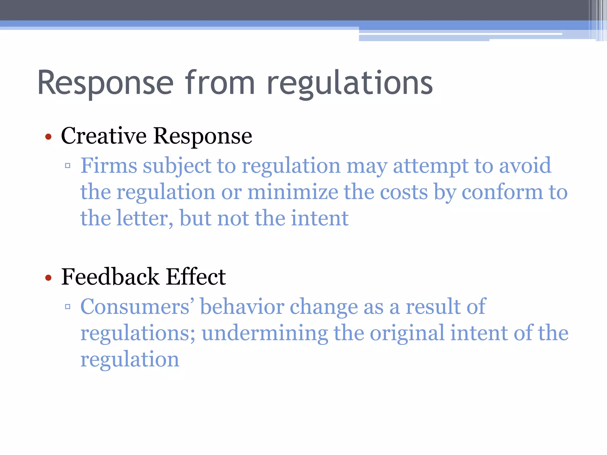
    Response from regulationsCreativeResponseFirms subject to regulation may attempt to avoid the regulation or minimize the costs by conform to the letter, but not the intentFeedback EffectConsumers’ behavior change as a result of regulations; undermining the original intent of the regulation
  • 5.
  • 6.
    Opportunity CostUSA1 computer= 0.5 wineItaly1 computer = 4 winesShould USA trade 1 computer for 4 wines from Italy?OrShould Italy trade 1 wine for 2 computers from USA?
  • 7.
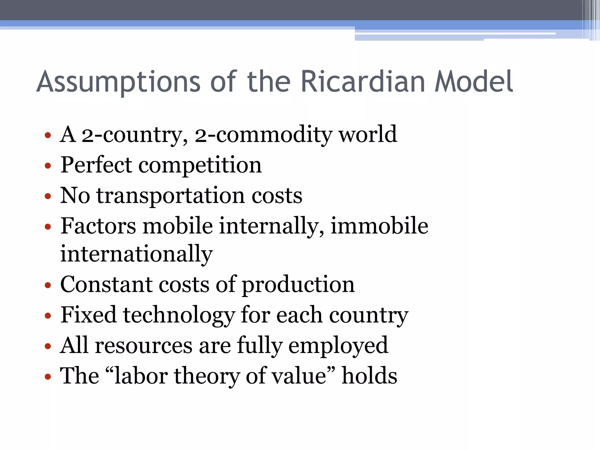
    Assumptions of theRicardian ModelA 2-country, 2-commodity worldPerfect competitionNo transportation costsFactors mobile internally, immobile internationallyConstant costs of productionFixed technology for each countryAll resources are fully employedThe “labor theory of value” holds
  • 8.
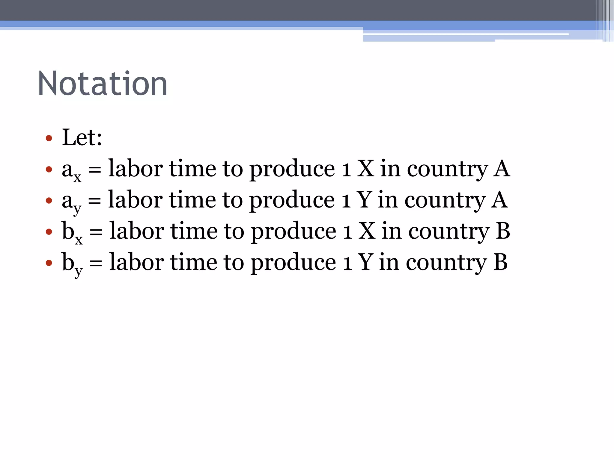
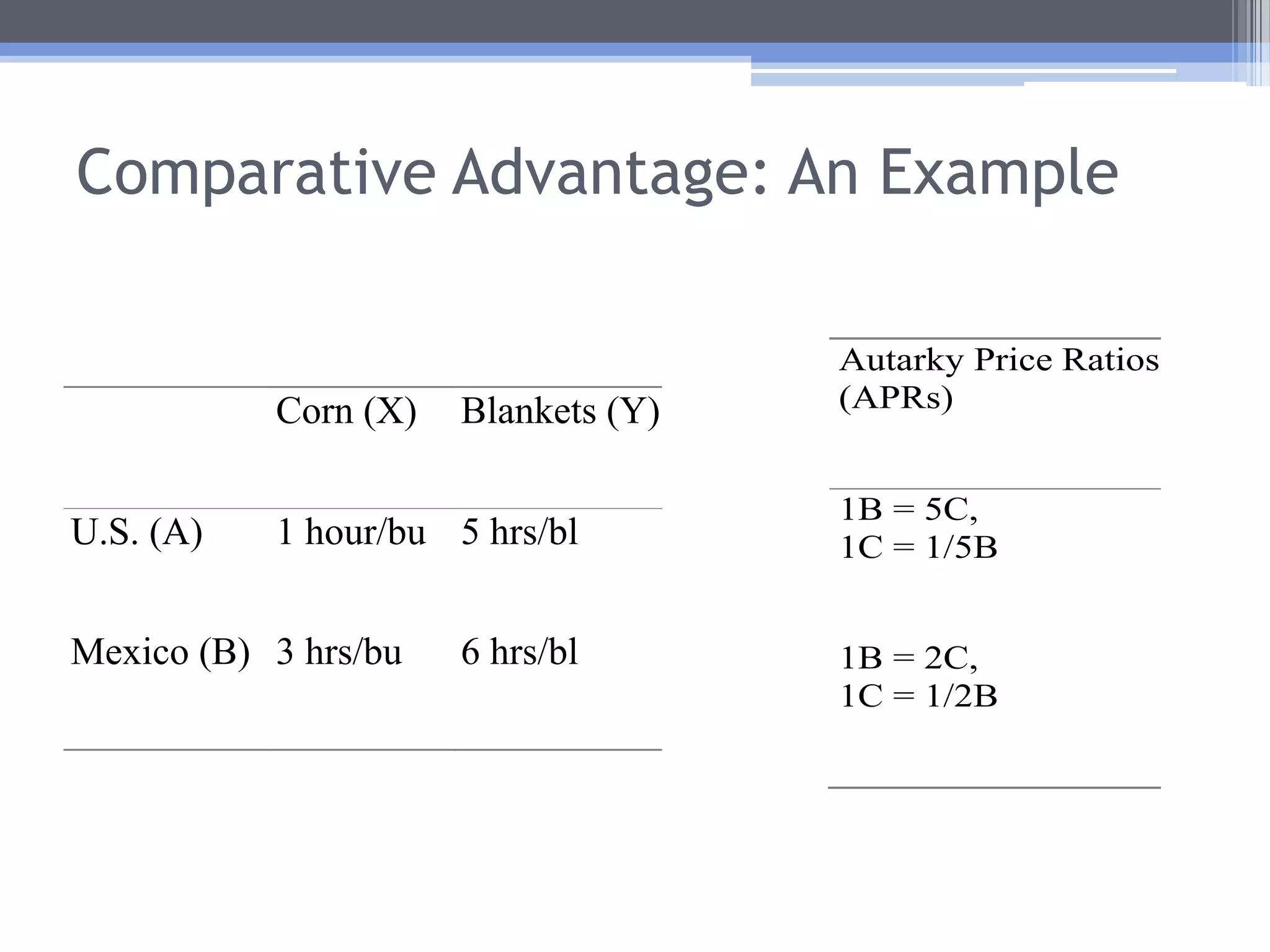
    NotationLet:ax = labortime to produce 1 X in country Aay = labor time to produce 1 Y in country Abx = labor time to produce 1 X in country Bby = labor time to produce 1 Y in country B
  • 9.
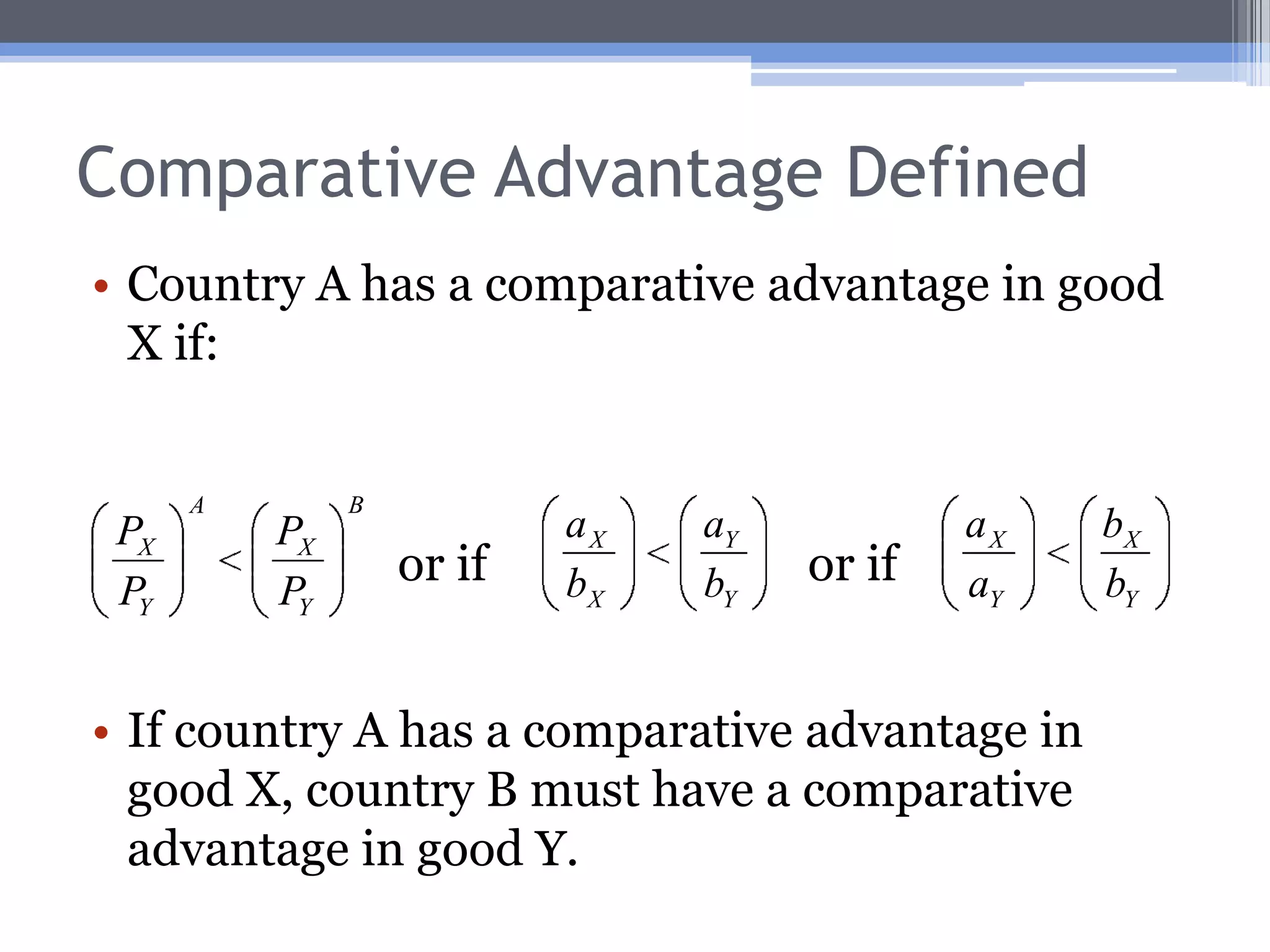
    Comparative Advantage DefinedCountryA has a comparative advantage in good X if:If country A has a comparative advantage in good X, country B must have a comparative advantage in good Y.or ifor if
  • 10.
  • 11.
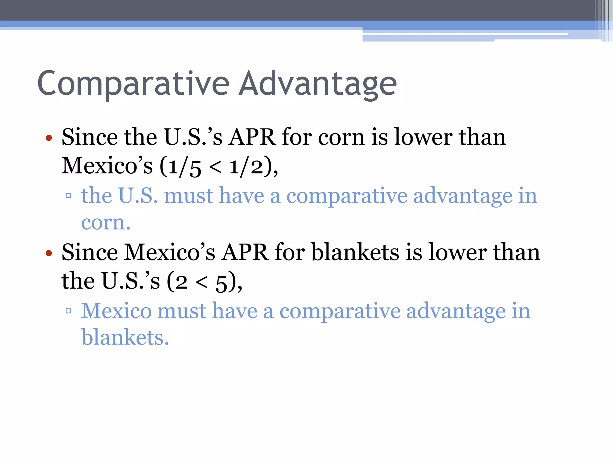
    Comparative AdvantageSince theU.S.’s APR for corn is lower than Mexico’s (1/5 < 1/2), the U.S. must have a comparative advantage in corn.Since Mexico’s APR for blankets is lower than the U.S.’s (2 < 5), Mexico must have a comparative advantage in blankets.
  • 12.
    Comparative Advantage andthe Total Gains from TradeRicardo’s argument is that trade will be mutually advantageous as long as the two countries’ autarky price ratios are different.How do we know that this is true?
  • 13.
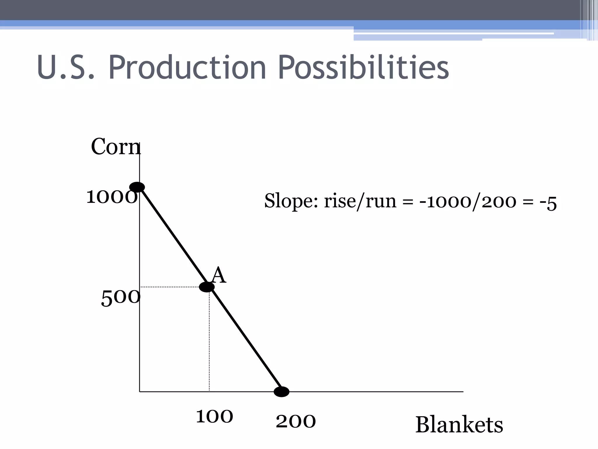
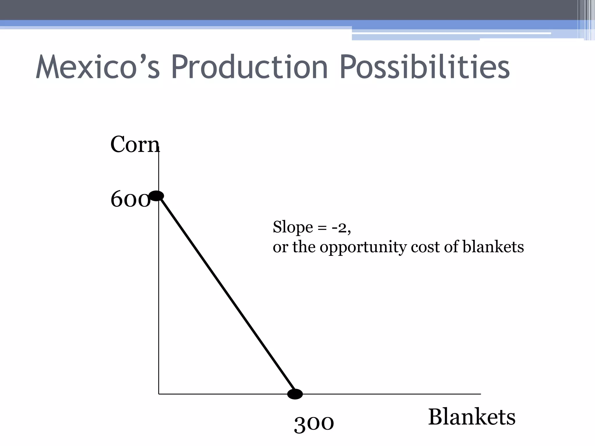
    Comparative Advantage andthe Total Gains from TradeThe Production Possibilities Frontier (PPF) is the set of all combinations of goods that a country is capable of producing, given available technology and resources.Suppose in our example the U.S. has 1,000 hours of labor available and Mexico has 1,800.
  • 14.
    U.S. Production PossibilitiesCorn1000Slope:rise/run = -1000/200 = -5A500100200Blankets
  • 15.
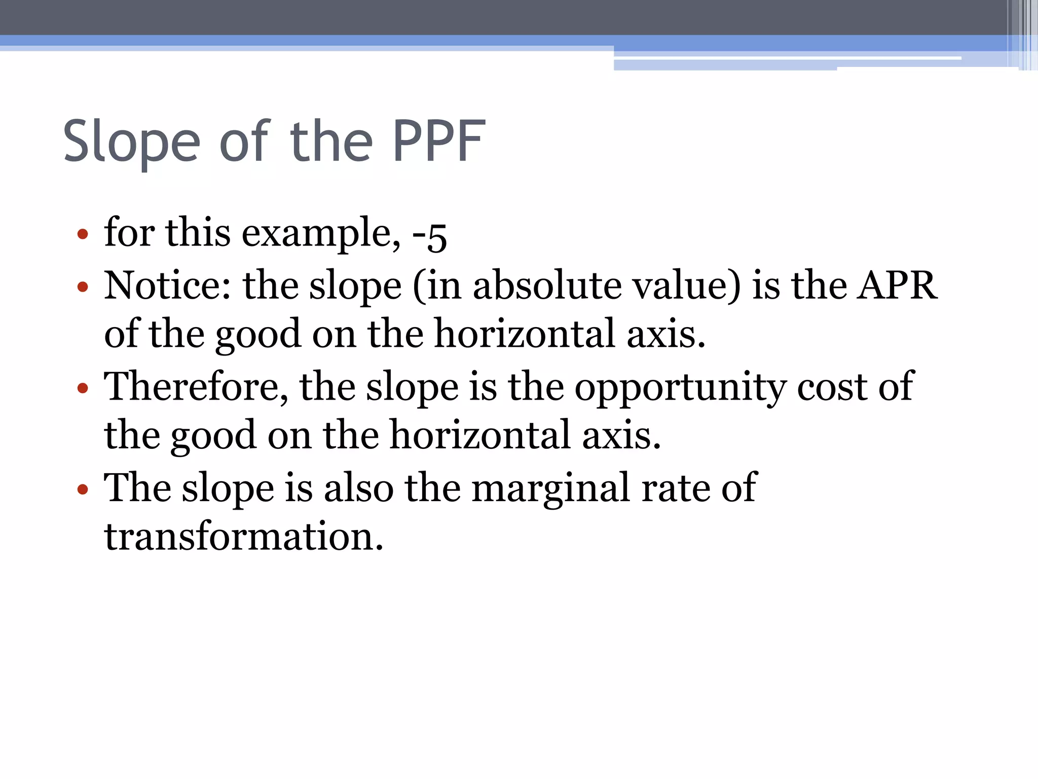
    Slope of thePPFfor this example, -5Notice: the slope (in absolute value) is the APR of the good on the horizontal axis.Therefore, the slope is the opportunity cost of the good on the horizontal axis.The slope is also the marginal rate of transformation.
  • 16.
    Mexico’s Production PossibilitiesCorn600Slope= -2, or the opportunity cost of blankets Blankets300
  • 17.
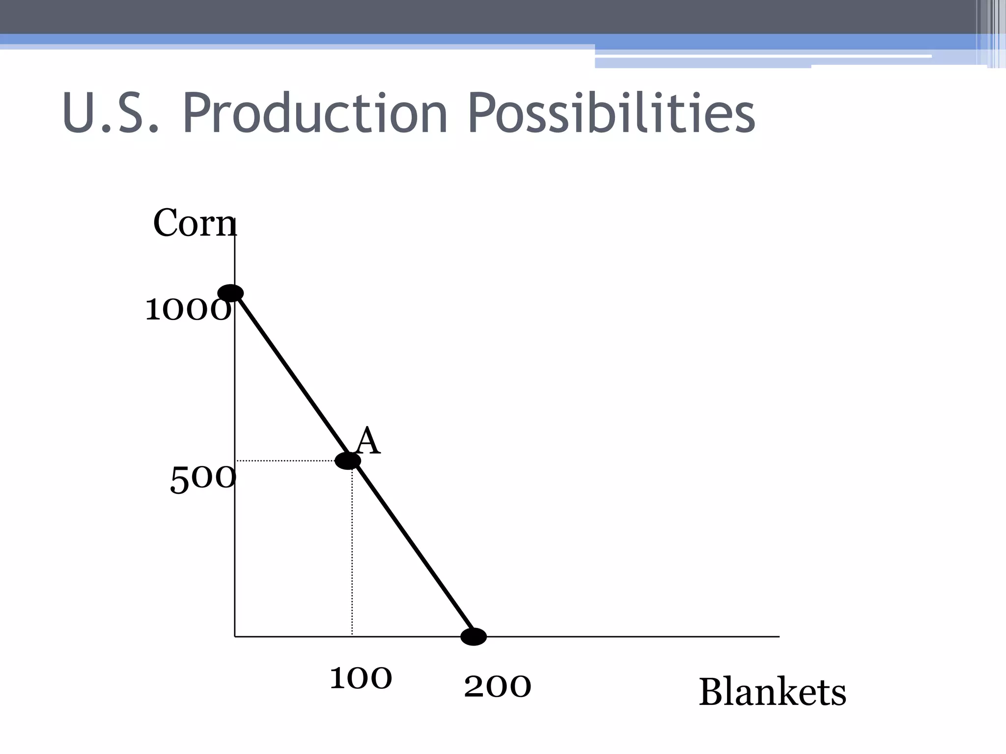
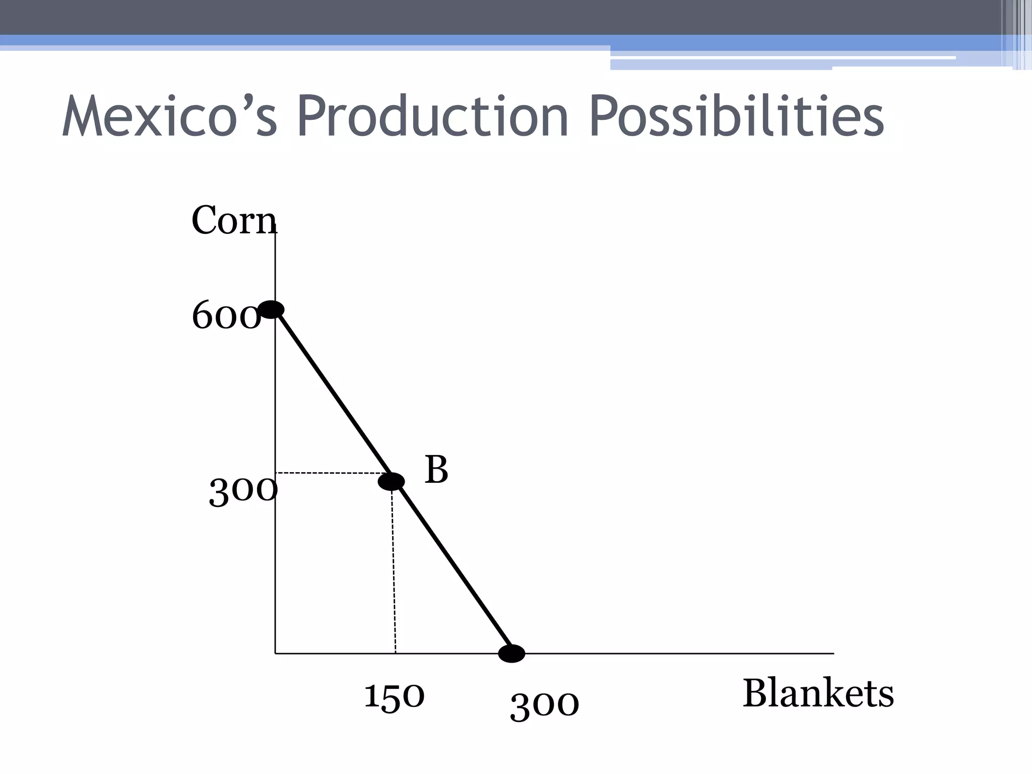
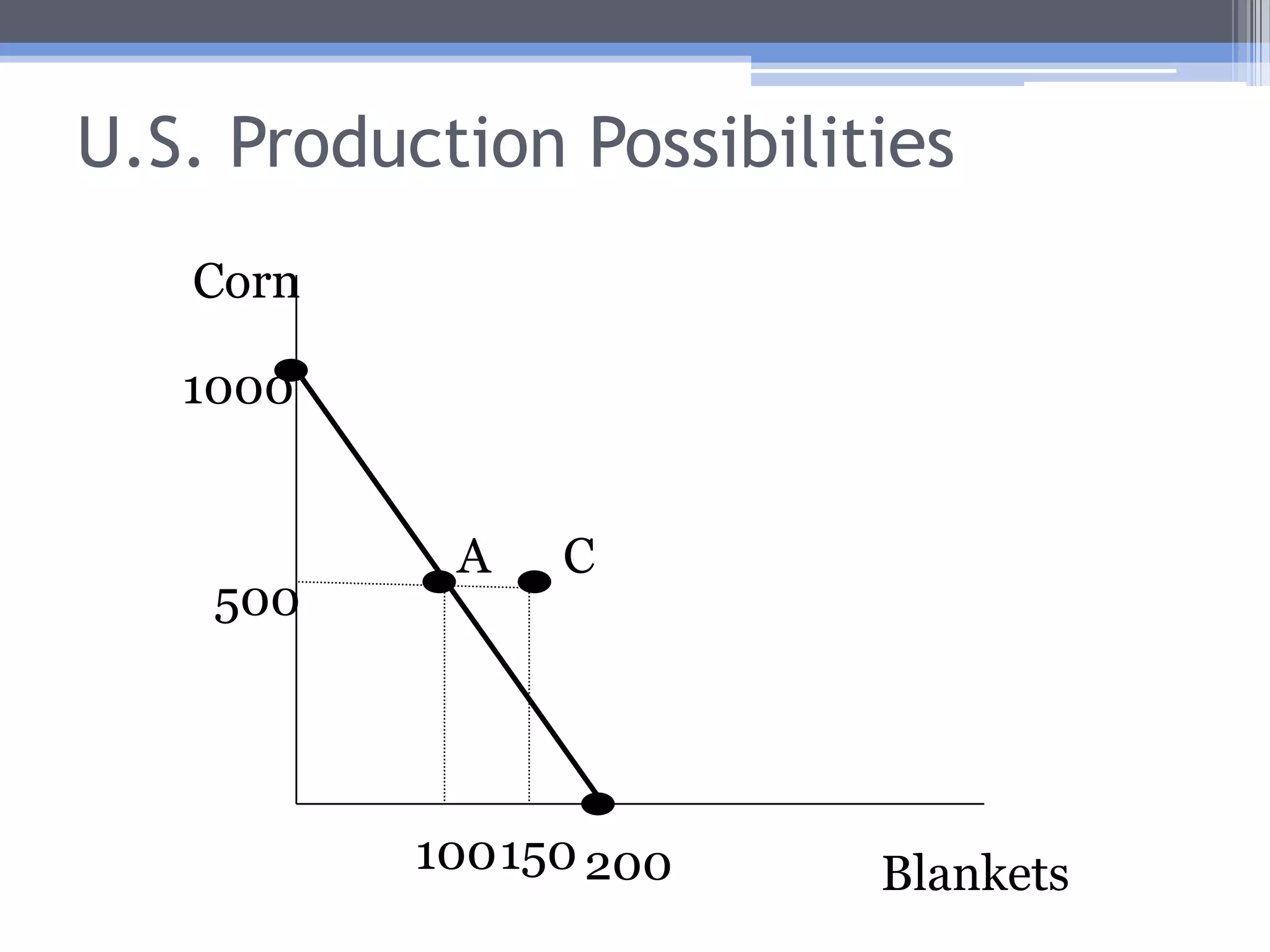
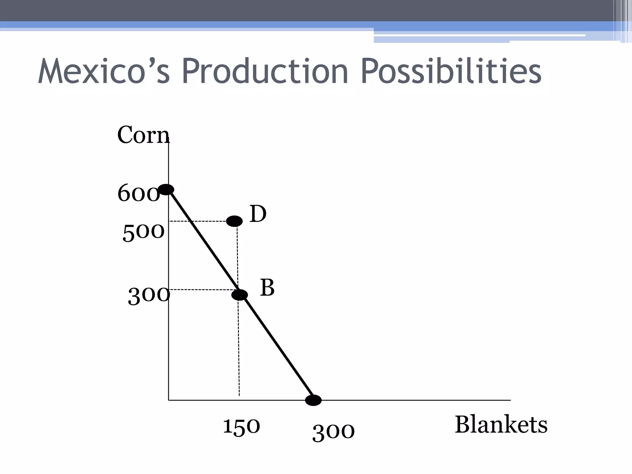
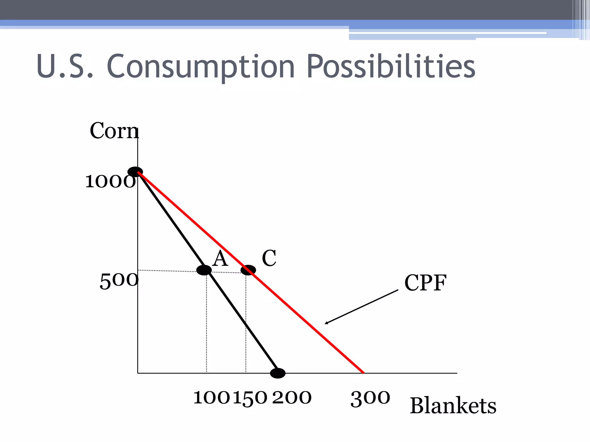
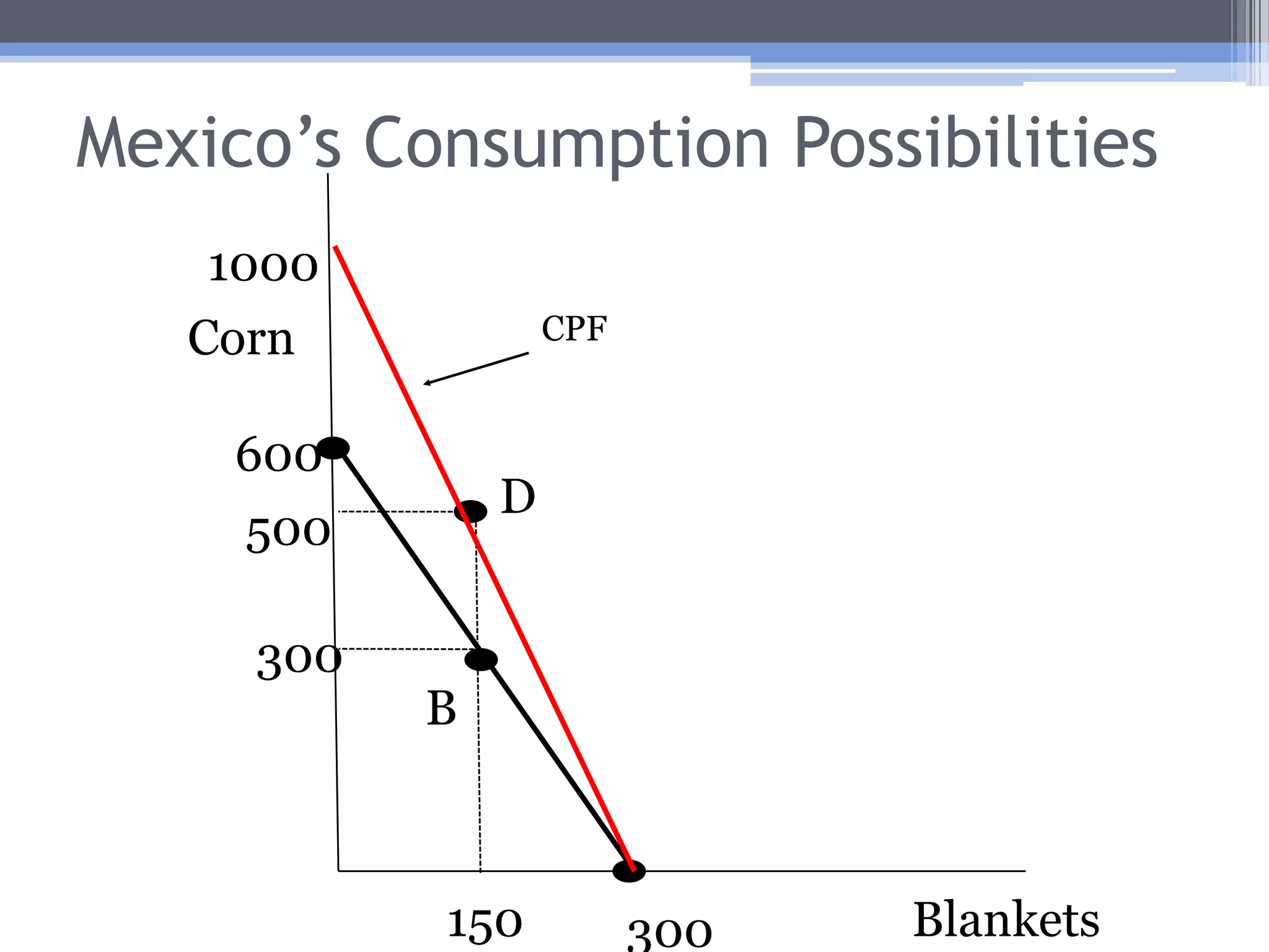
    Classical Model: TheGains from TradeSuppose that in autarkythe U.S. is at point AProducing 500 corn Consuming 100 blanketsMexico is at point BProducing 300 corn Consuming 150 blankets
  • 18.
  • 19.
  • 20.
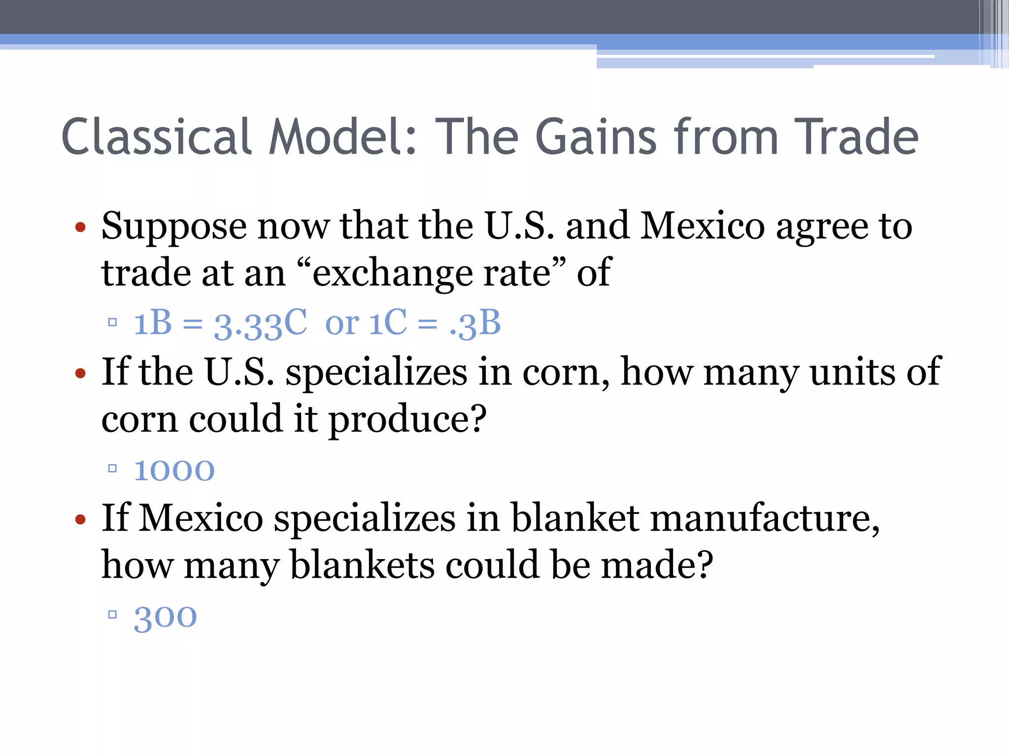
    Classical Model: TheGains from TradeSuppose now that the U.S. and Mexico agree to trade at an “exchange rate” of 1B = 3.33C or 1C = .3BIf the U.S. specializes in corn, how many units of corn could it produce? 1000If Mexico specializes in blanket manufacture, how many blankets could be made? 300
  • 21.
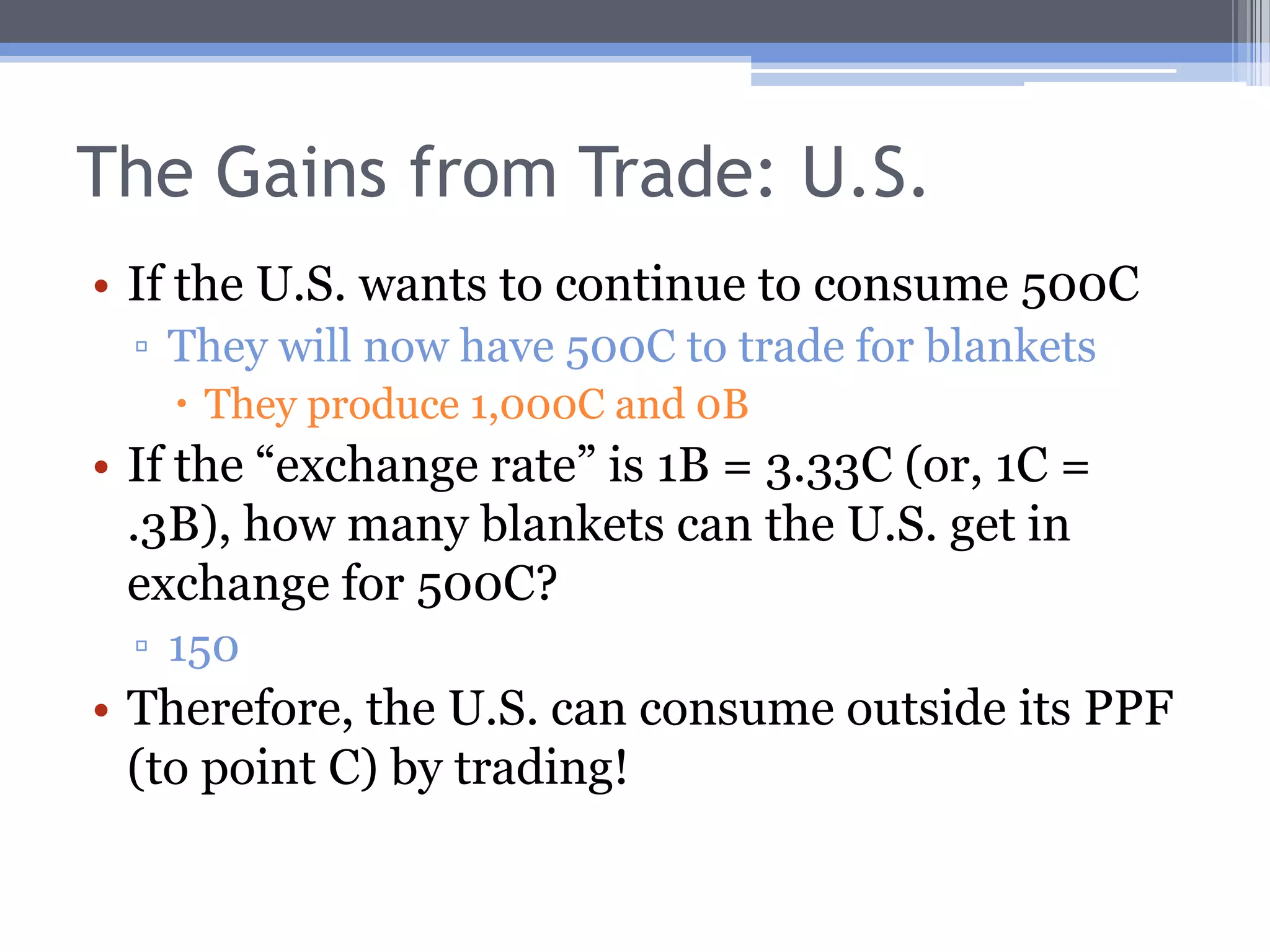
    The Gains fromTrade: U.S.If the U.S. wants to continue to consume 500CThey will now have 500C to trade for blanketsThey produce 1,000C and 0BIf the “exchange rate” is 1B = 3.33C (or, 1C = .3B), how many blankets can the U.S. get in exchange for 500C?150Therefore, the U.S. can consume outside its PPF (to point C) by trading!
  • 22.
  • 23.
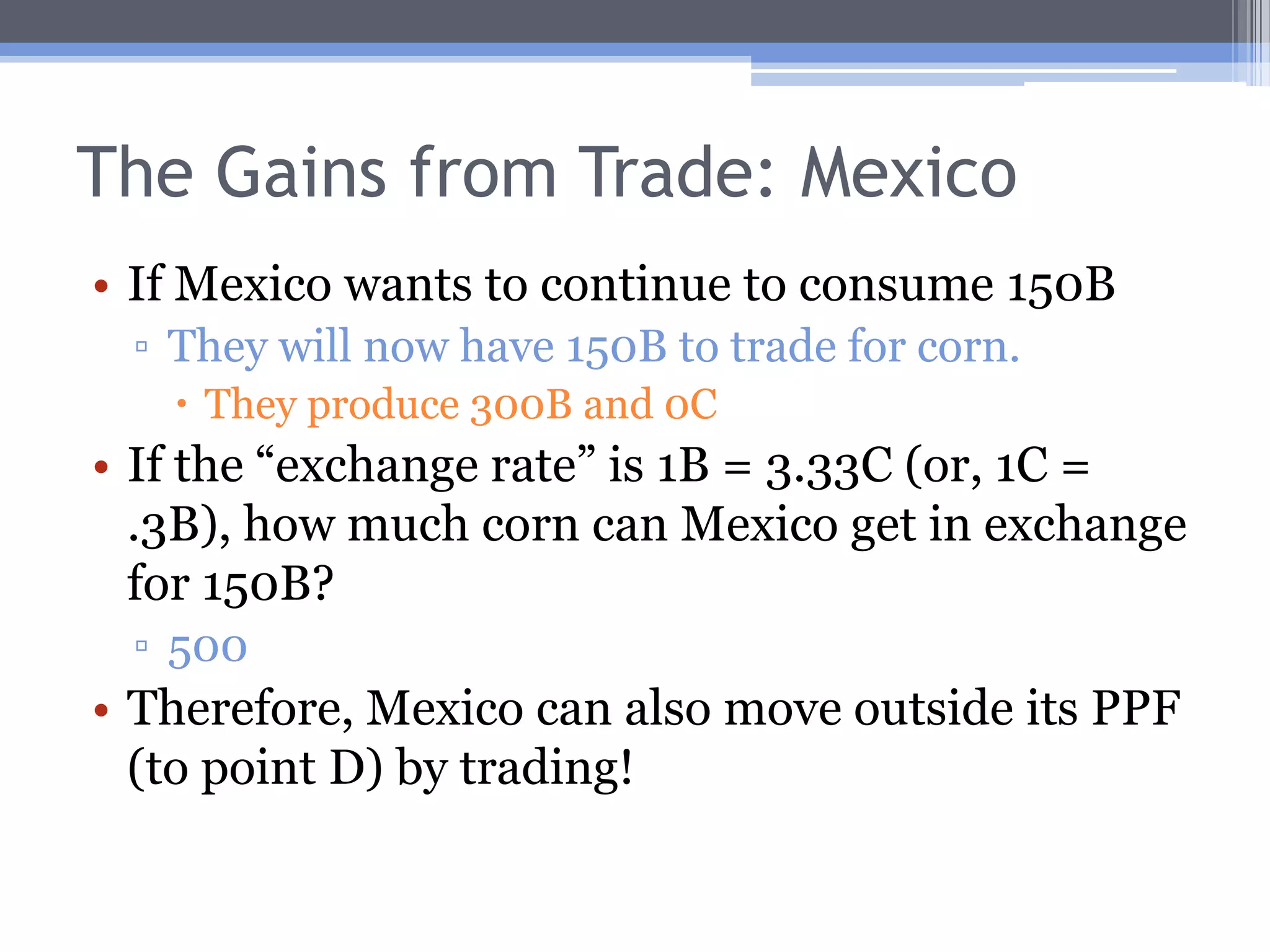
    The Gains fromTrade: MexicoIf Mexico wants to continue to consume 150BThey will now have 150B to trade for corn.They produce 300B and 0CIf the “exchange rate” is 1B = 3.33C (or, 1C = .3B), how much corn can Mexico get in exchange for 150B?500Therefore, Mexico can also move outside its PPF (to point D) by trading!
  • 24.
  • 25.
    The Gains fromTradeNote: In generalThe Ricardian model results in complete specialization.However, in trade between a small and a large country the small country may not be able to produce enough to satisfy the large country; the large country might then partially specialize.
  • 26.
    The Consumption PossibilitiesFrontier (CPF)The CPF is a collection of points that represent combinations of corn and blankets that a country can consume if it trades.
  • 27.
  • 28.
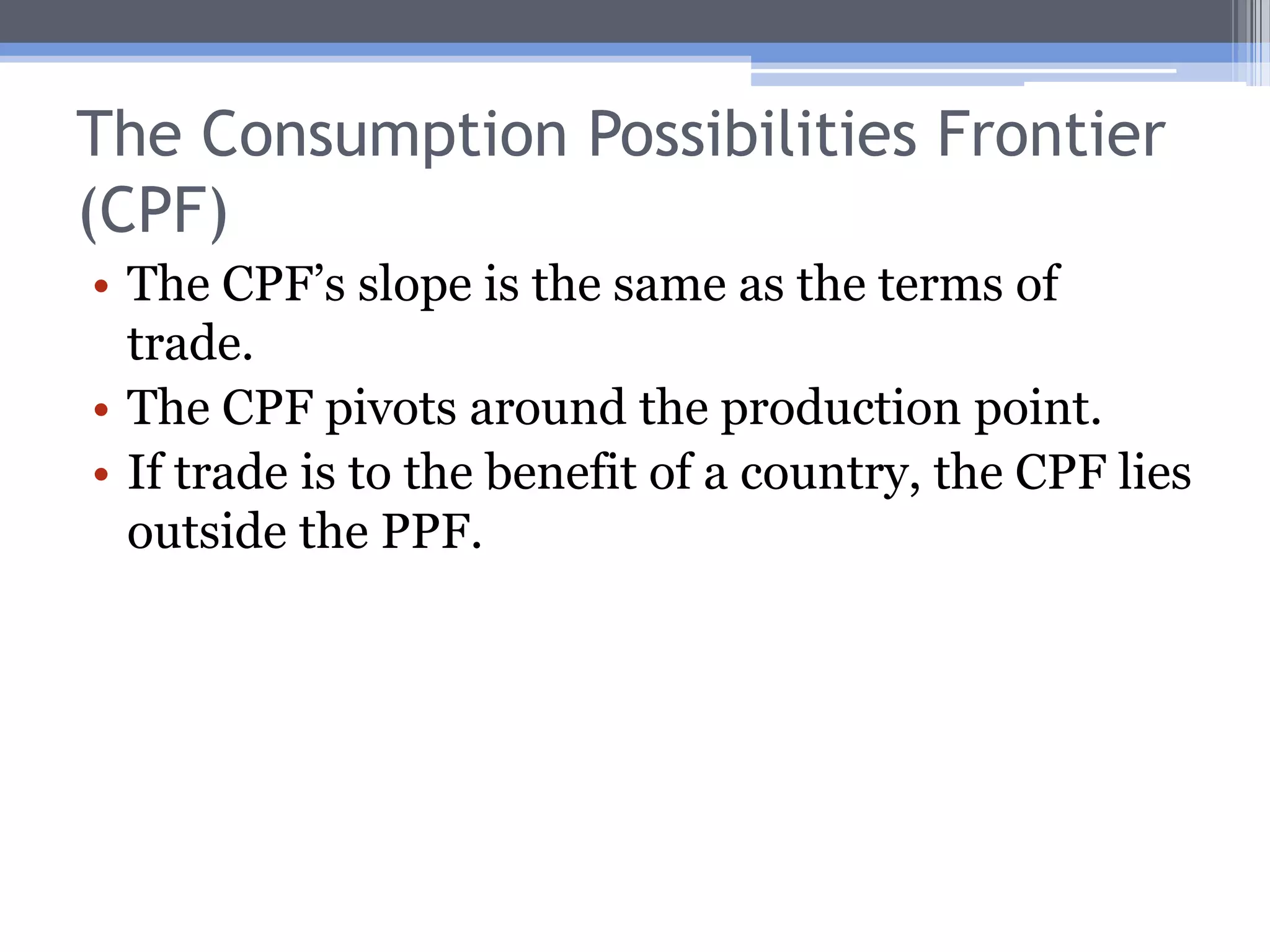
    The Consumption PossibilitiesFrontier (CPF)The CPF’s slope is the same as the terms of trade.The CPF pivots around the production point.If trade is to the benefit of a country, the CPF lies outside the PPF.
  • 29.
  • 30.
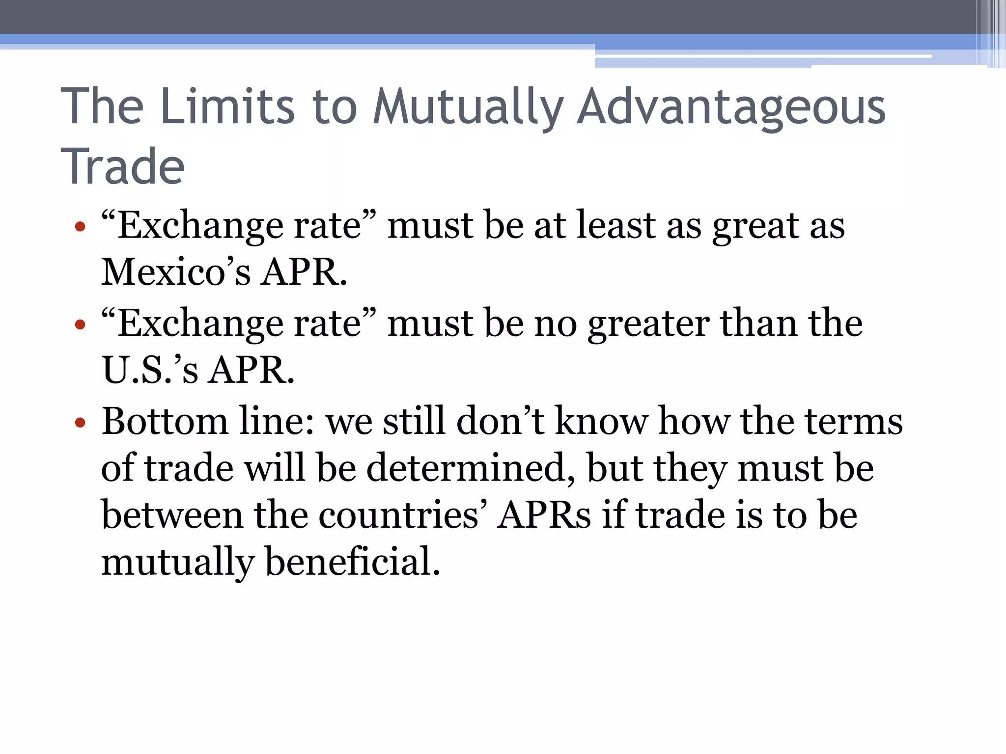
    The Limits toMutually Advantageous Trade“Exchange rate” must be at least as great as Mexico’s APR.“Exchange rate” must be no greater than the U.S.’s APR.Bottom line: we still don’t know how the terms of trade will be determined, but they must be between the countries’ APRs if trade is to be mutually beneficial.
  • 31.
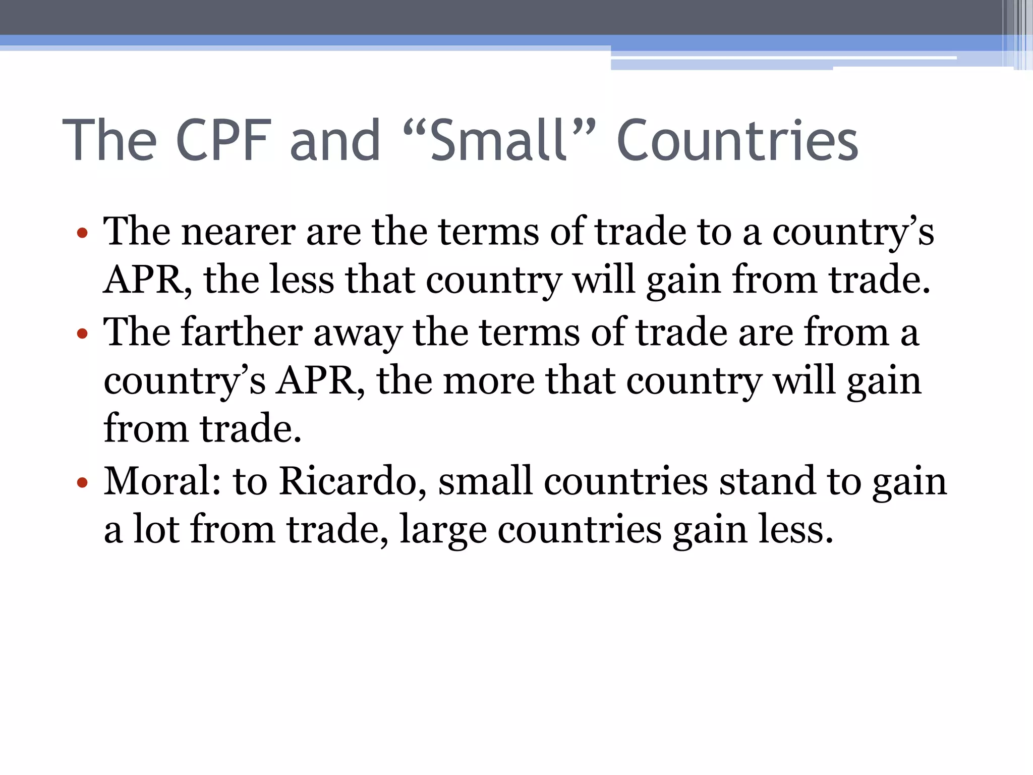
    The CPF and“Small” CountriesThe nearer are the terms of trade to a country’s APR, the less that country will gain from trade.The farther away the terms of trade are from a country’s APR, the more that country will gain from trade.Moral: to Ricardo, small countries stand to gain a lot from trade, large countries gain less.
  • 32.
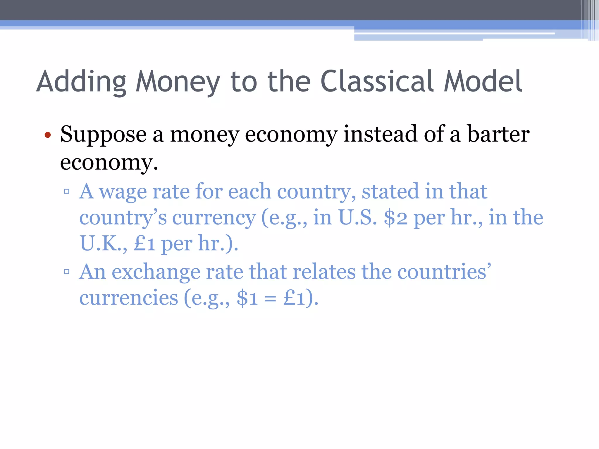
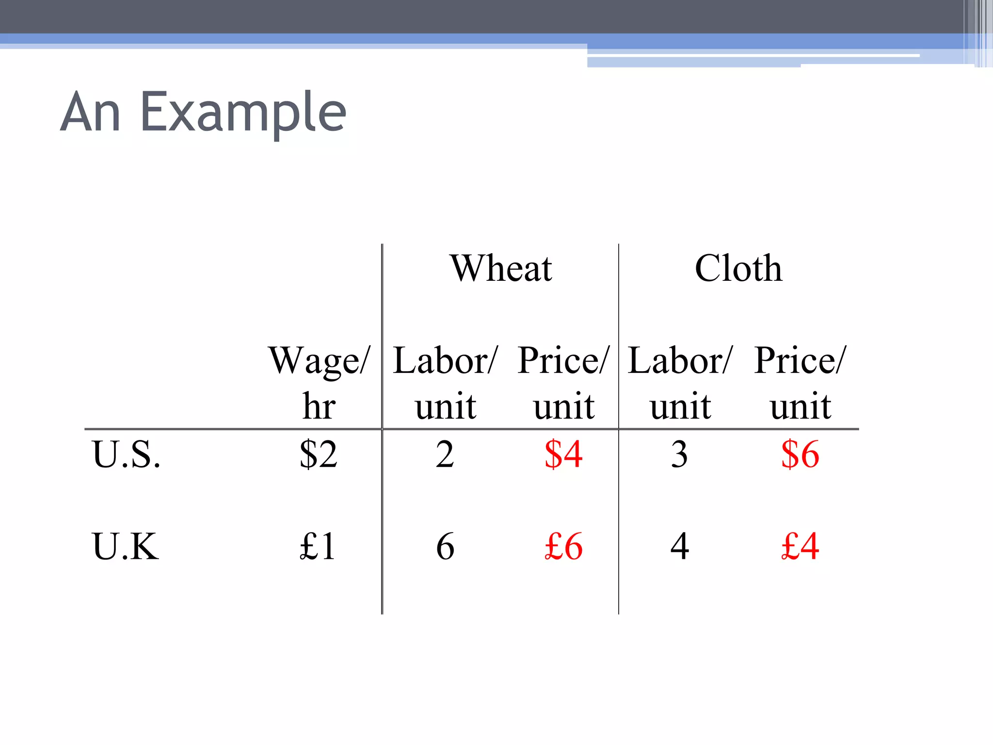
    Adding Money tothe Classical ModelSuppose a money economy instead of a barter economy.A wage rate for each country, stated in that country’s currency (e.g., in U.S. $2 per hr., in the U.K., £1 per hr.).An exchange rate that relates the countries’ currencies (e.g., $1 = £1).
  • 33.
  • 34.
  • 35.
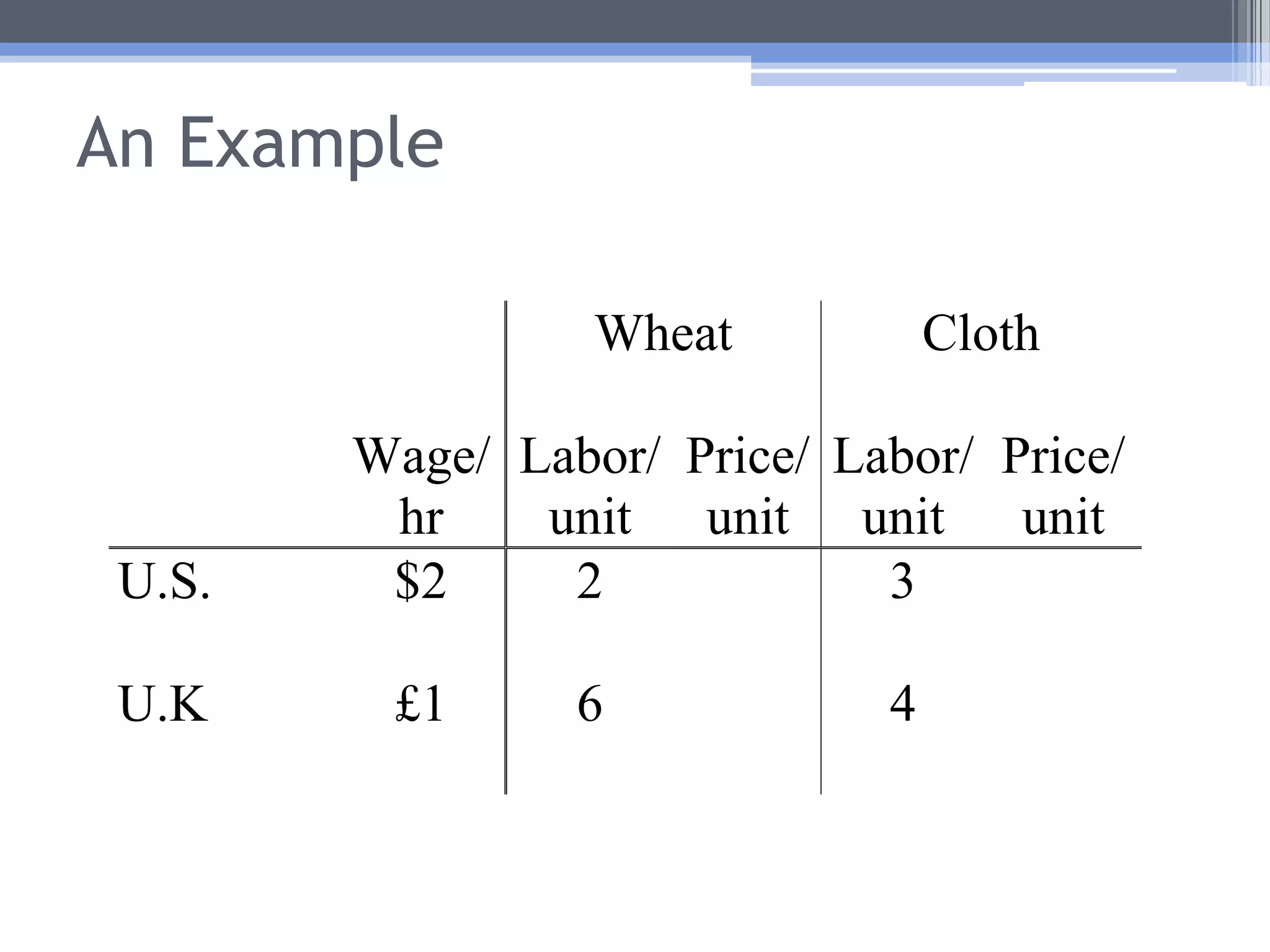
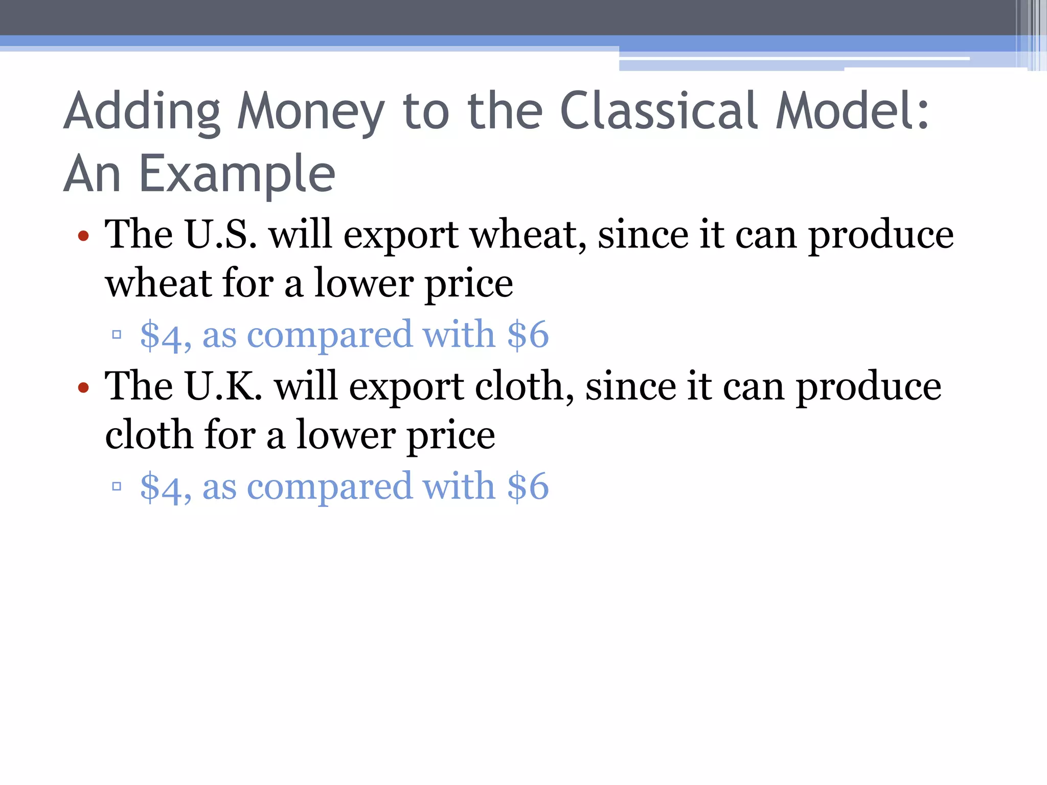
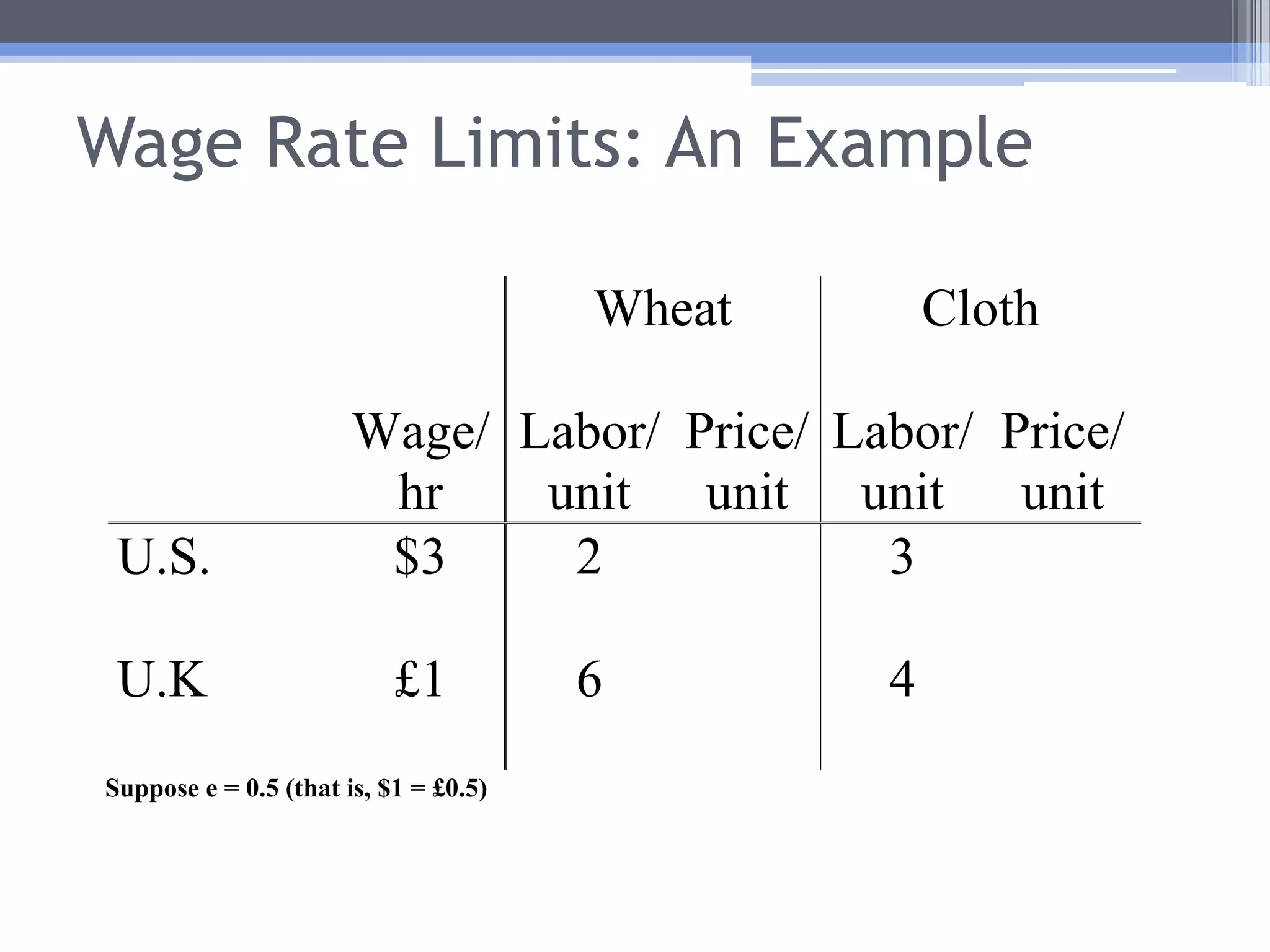
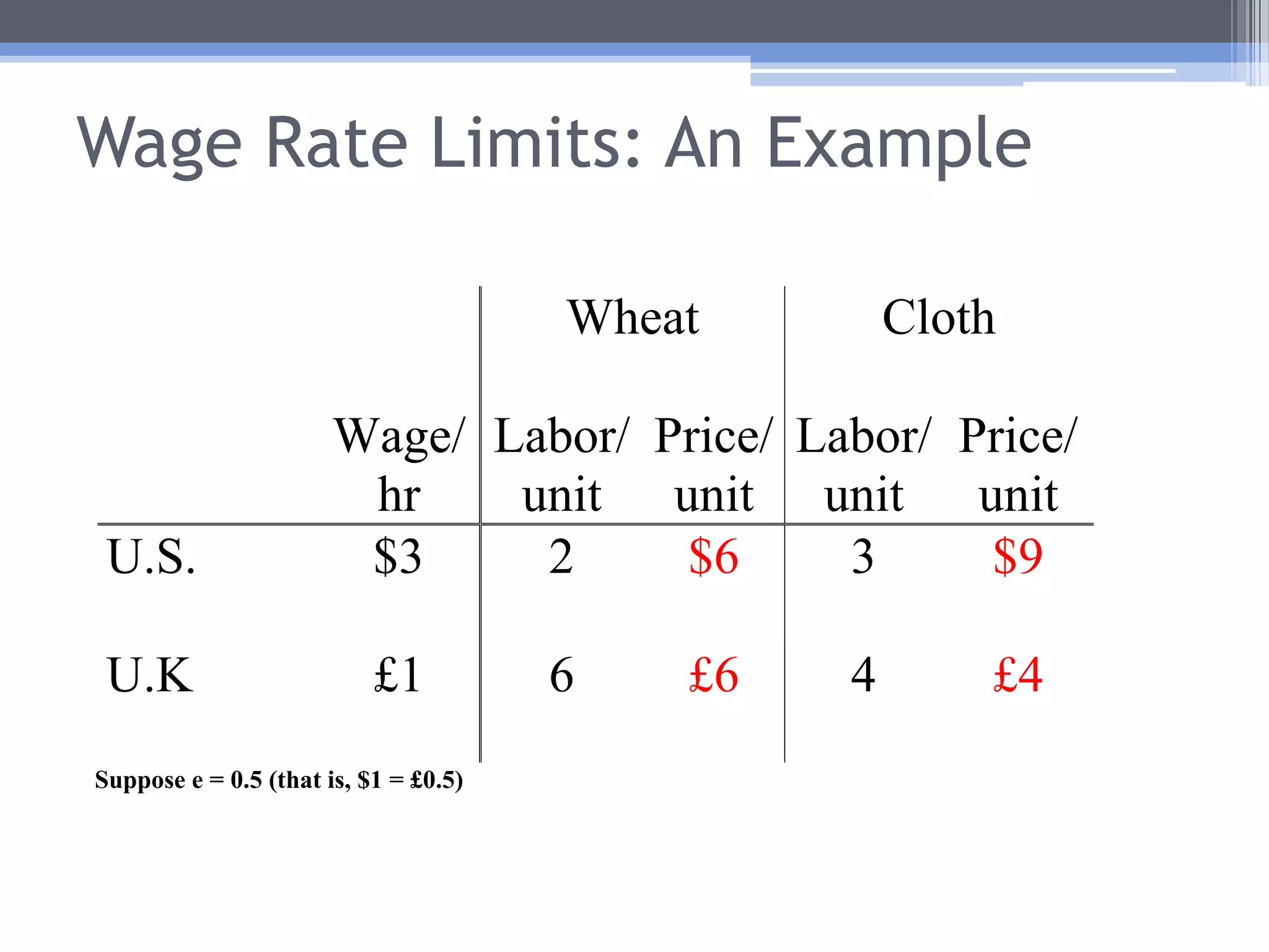
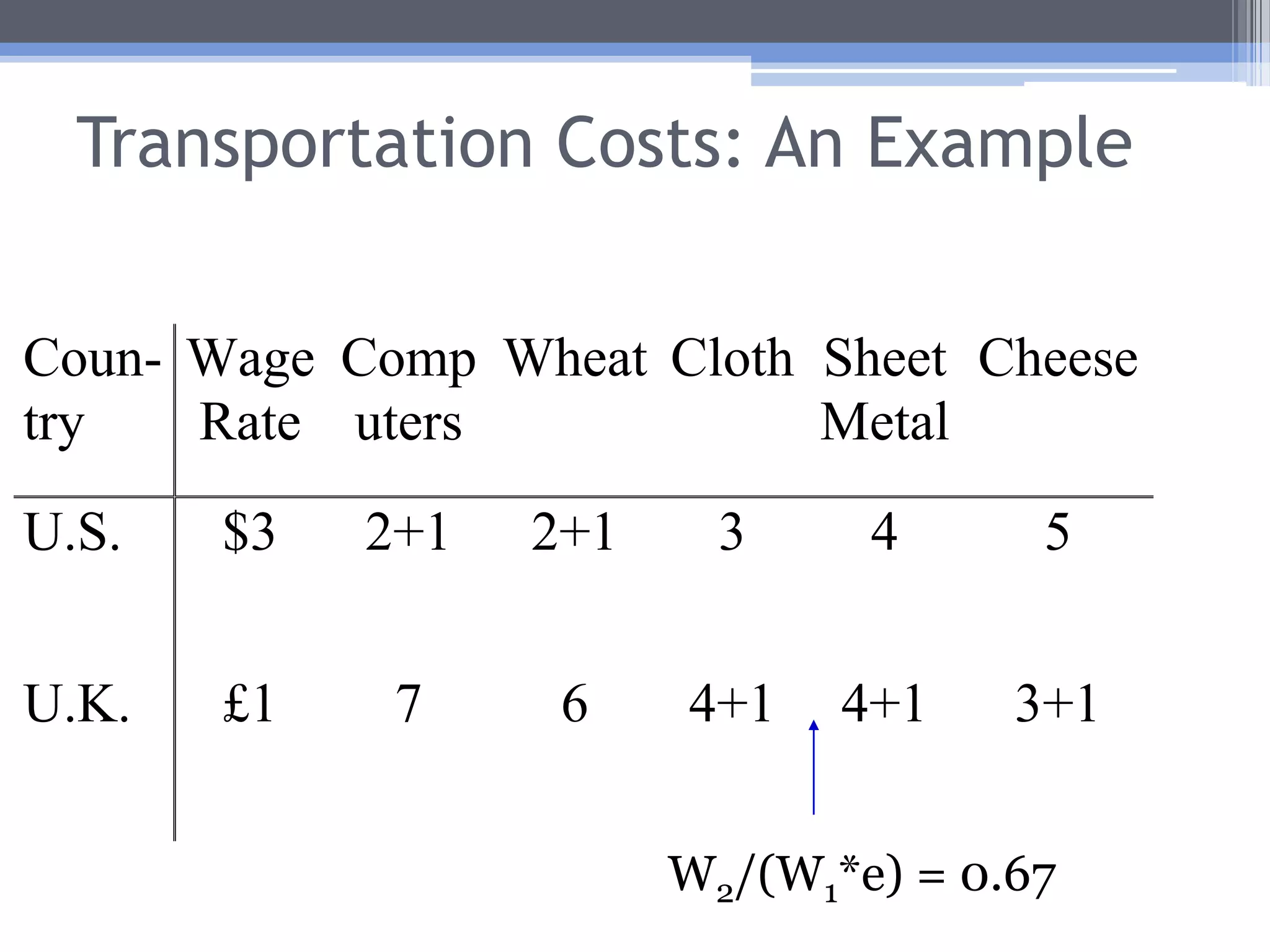
    Adding Money tothe Classical Model: An ExampleThe U.S. will export wheat, since it can produce wheat for a lower price $4, as compared with $6The U.K. will export cloth, since it can produce cloth for a lower price $4, as compared with $6
  • 36.
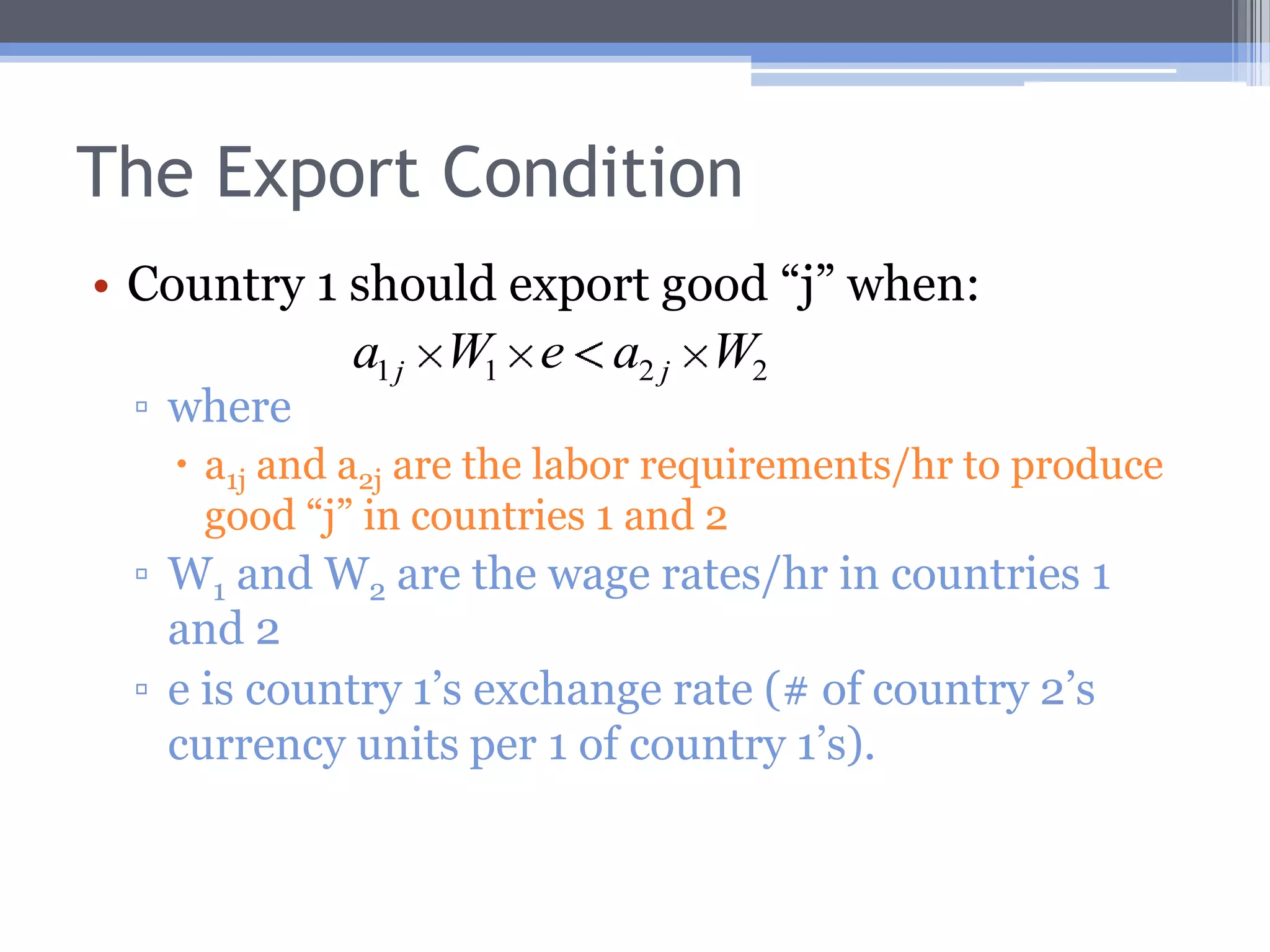
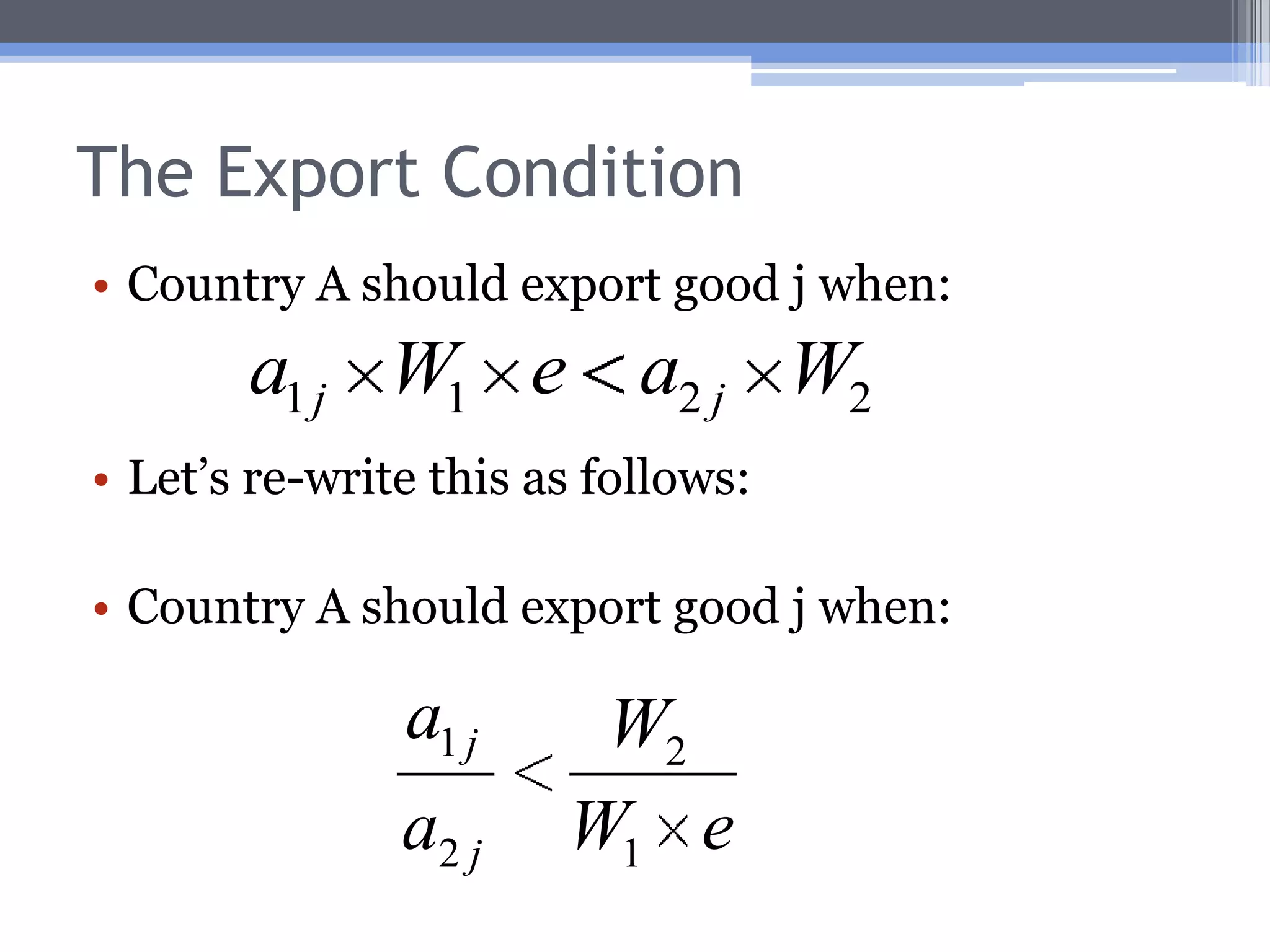
    The Export ConditionCountry1 should export good “j” when: wherea1j and a2j are the labor requirements/hr to produce good “j” in countries 1 and 2W1 and W2 are the wage rates/hr in countries 1 and 2e is country 1’s exchange rate (# of country 2’s currency units per 1 of country 1’s).
  • 37.
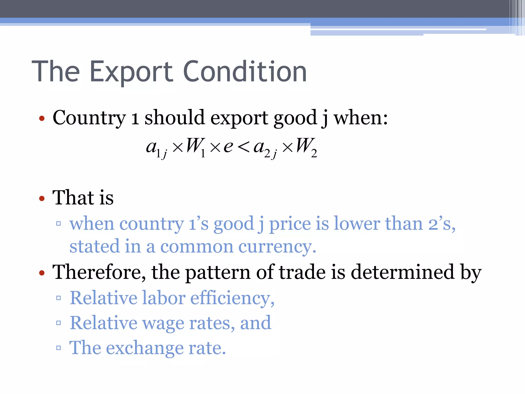
    The Export ConditionCountry1 should export good j when: That iswhen country 1’s good j price is lower than 2’s, stated in a common currency.Therefore, the pattern of trade is determined byRelative labor efficiency,Relative wage rates, andThe exchange rate.
  • 38.
    The Export ConditionCountryA should export good j when: Let’s re-write this as follows:Country A should export good j when:
  • 39.
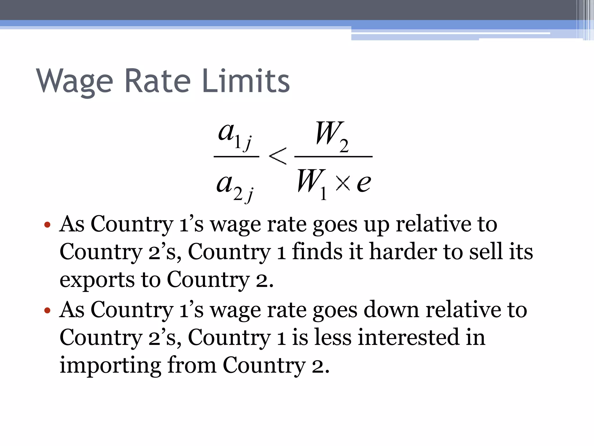
    Wage Rate LimitsAsCountry 1’s wage rate goes up relative to Country 2’s, Country 1 finds it harder to sell its exports to Country 2.As Country 1’s wage rate goes down relative to Country 2’s, Country 1 is less interested in importing from Country 2.
  • 40.
  • 41.
  • 42.
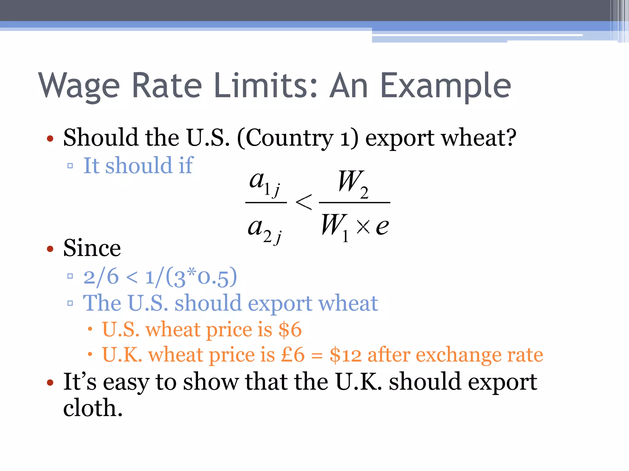
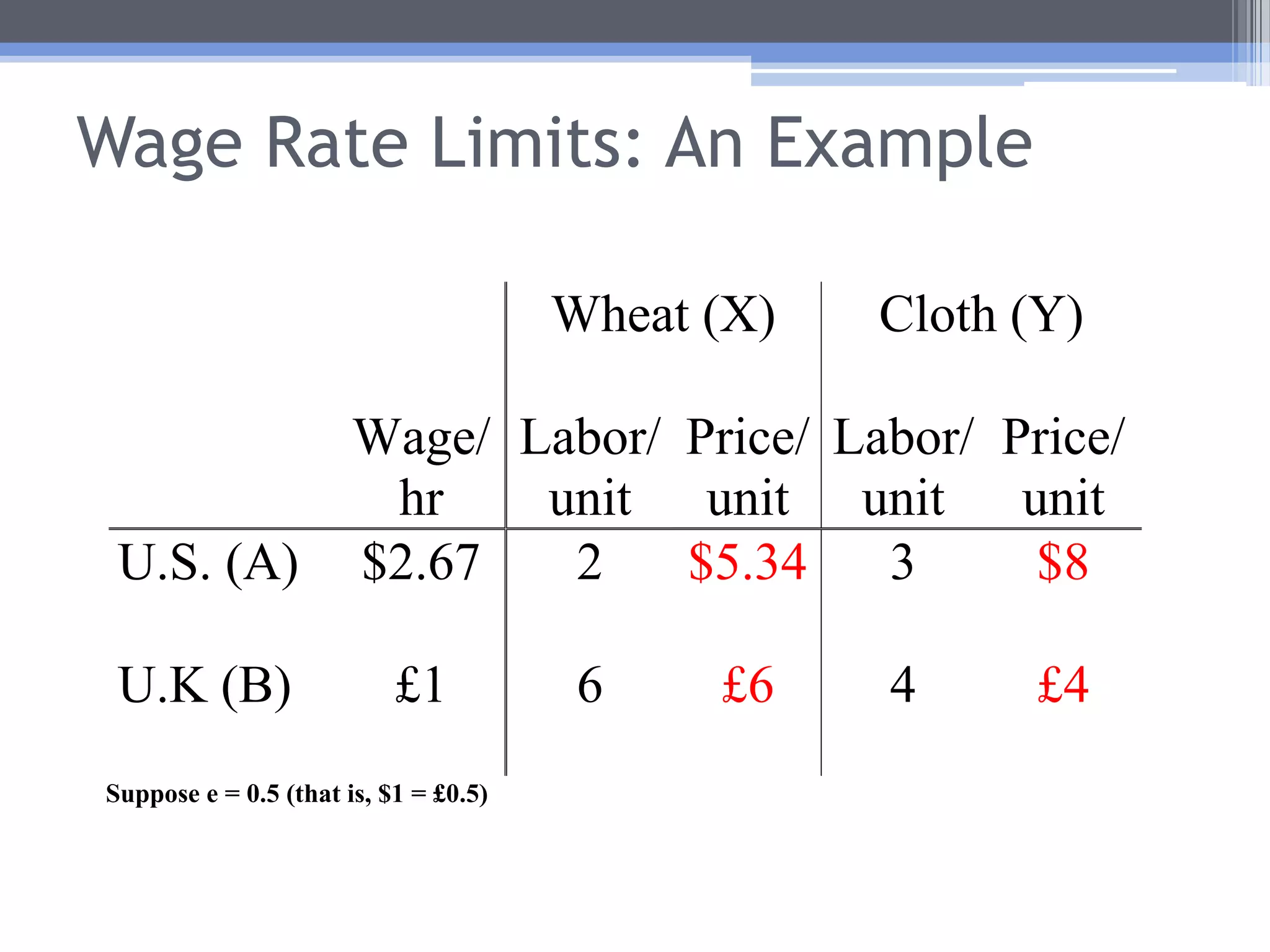
    Wage Rate Limits:An ExampleShould the U.S. (Country 1) export wheat? It should ifSince 2/6 < 1/(3*0.5)The U.S. should export wheat U.S. wheat price is $6U.K. wheat price is £6 = $12 after exchange rateIt’s easy to show that the U.K. should export cloth.
  • 43.
    Wage Rate Limits:An ExampleWhat if the U.S. wage rate rose to $6?
  • 44.
  • 45.
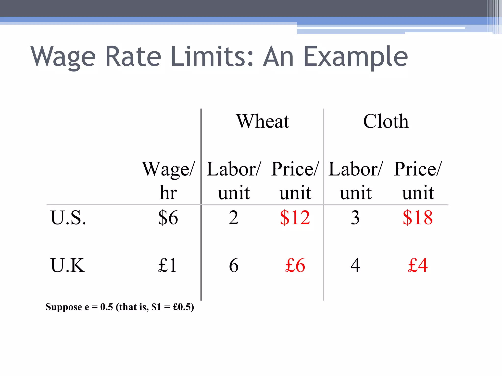
    Wage Rate Limits:An ExampleNow the U.S. wheat price is the same as the U.K.’s, if we state them in a common currency.Exchange rate: £1 = $2Therefore, If the wage rate in the U.S. should rise above $6, the U.K. will no longer buy U.S. wheat (trade will cease).
  • 46.
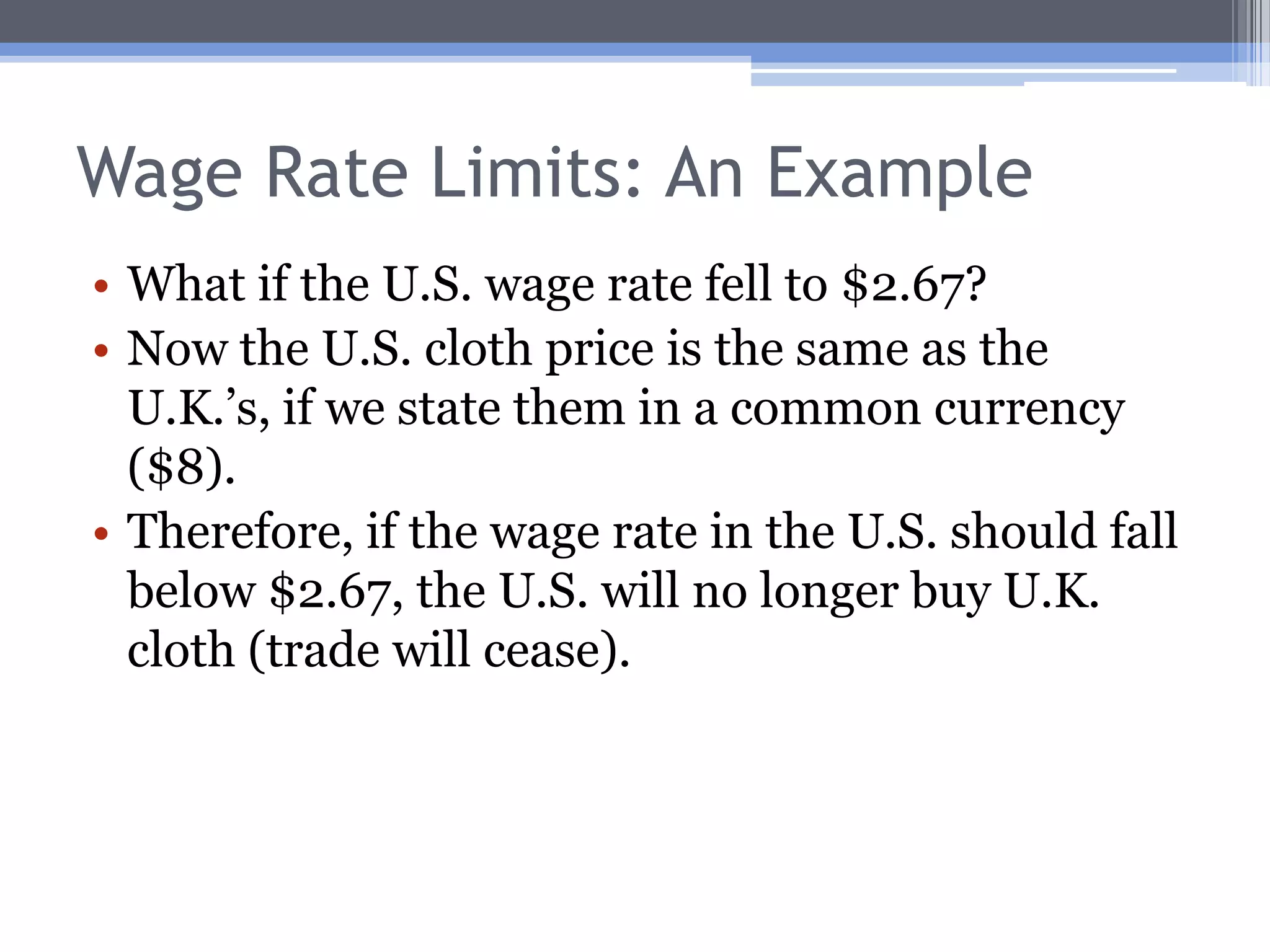
    Wage Rate Limits:An ExampleWhat if instead the U.S. wage rate fell to $2.67?
  • 47.
  • 48.
    Wage Rate Limits:An ExampleWhat if the U.S. wage rate fell to $2.67?Now the U.S. cloth price is the same as the U.K.’s, if we state them in a common currency ($8).Therefore, if the wage rate in the U.S. should fall below $2.67, the U.S. will no longer buy U.K. cloth (trade will cease).
  • 49.
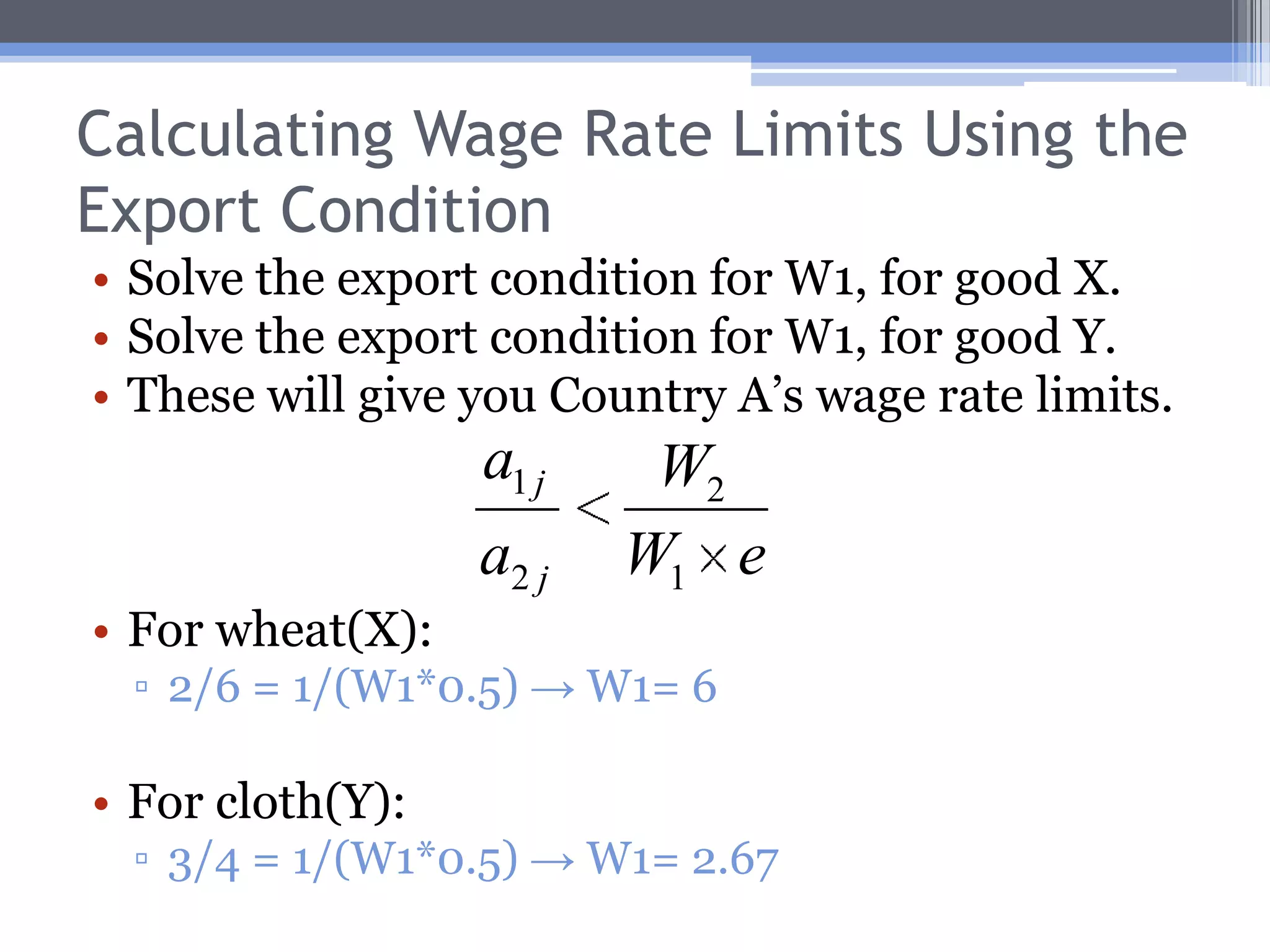
    Calculating Wage RateLimits Using the Export ConditionSolve the export condition for W1, for good X.Solve the export condition for W1, for good Y.These will give you Country A’s wage rate limits.For wheat(X):2/6 = 1/(W1*0.5) -> W1= 6For cloth(Y):3/4 = 1/(W1*0.5) -> W1= 2.67
  • 50.
    Country 2’s WageRate LimitsChanges in Country 2’s wage rates also can affect the pattern of trade.If 2’s wage rises too much, they will not be able to export any more.If 2’s wage falls too much, 2 will no longer wish to import.
  • 51.
    Exchange Rate LimitsIfCountry 1’s currency appreciatesImports will seem cheaper and exports more expensive.If 1’s currency appreciates enoughA will no longer be able to export.If 1’s currency depreciates enoughA will no longer wish to import.
  • 52.
    More Than TwoGoodsHaving more than two goods has no effect on the basic Classical model.The export condition can still be used.
  • 53.
    More Than TwoGoods: An Example
  • 54.
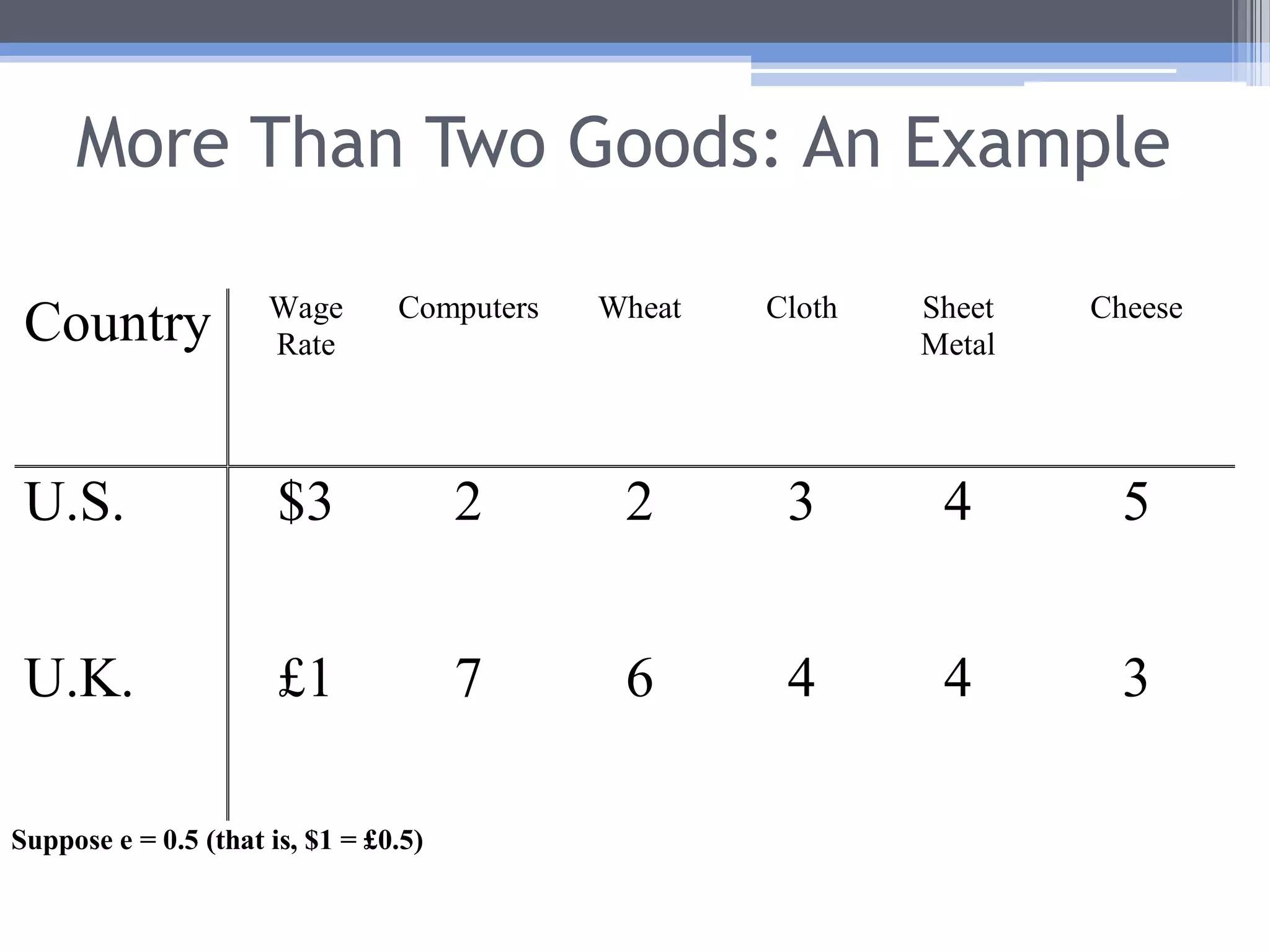
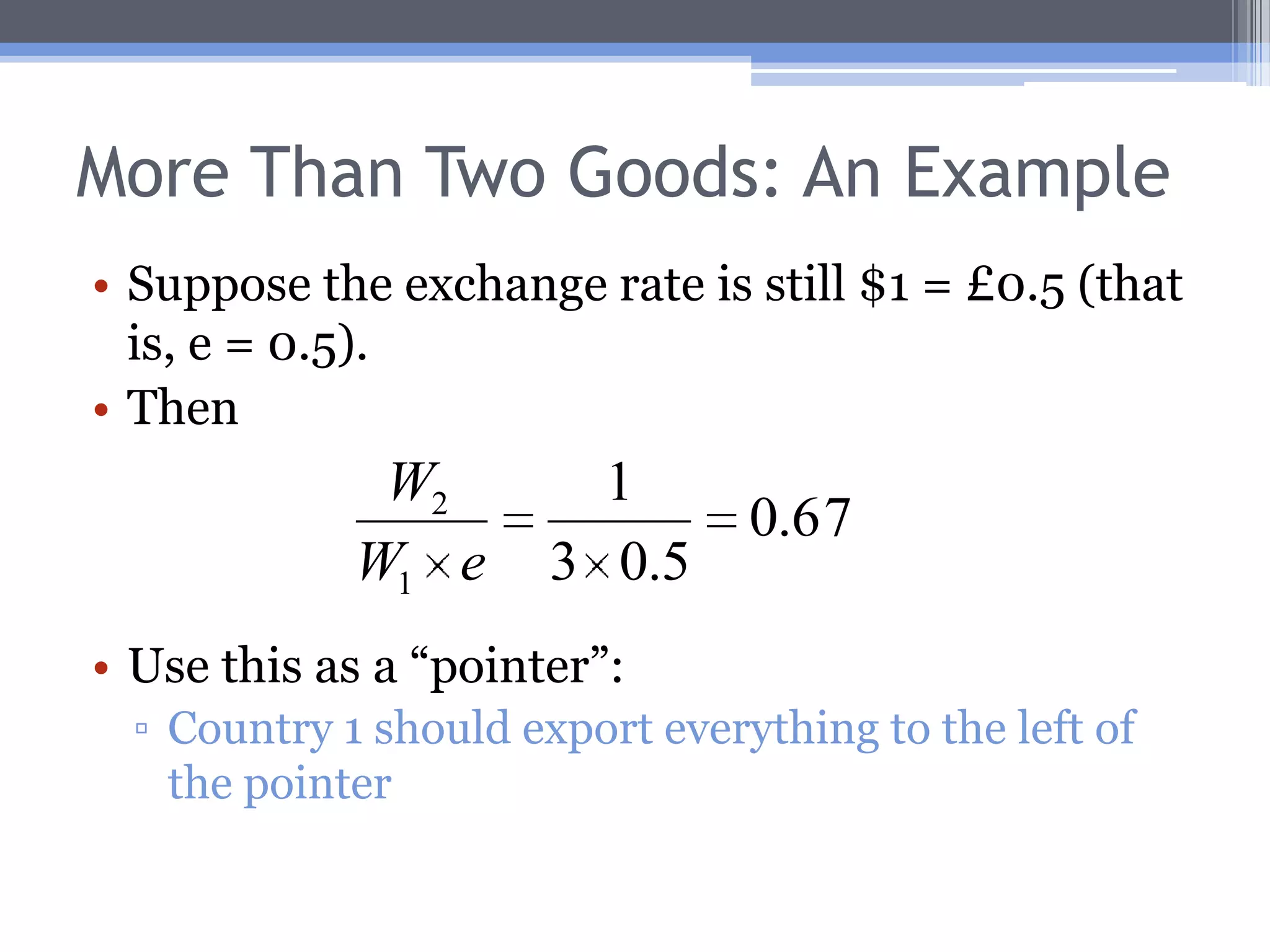
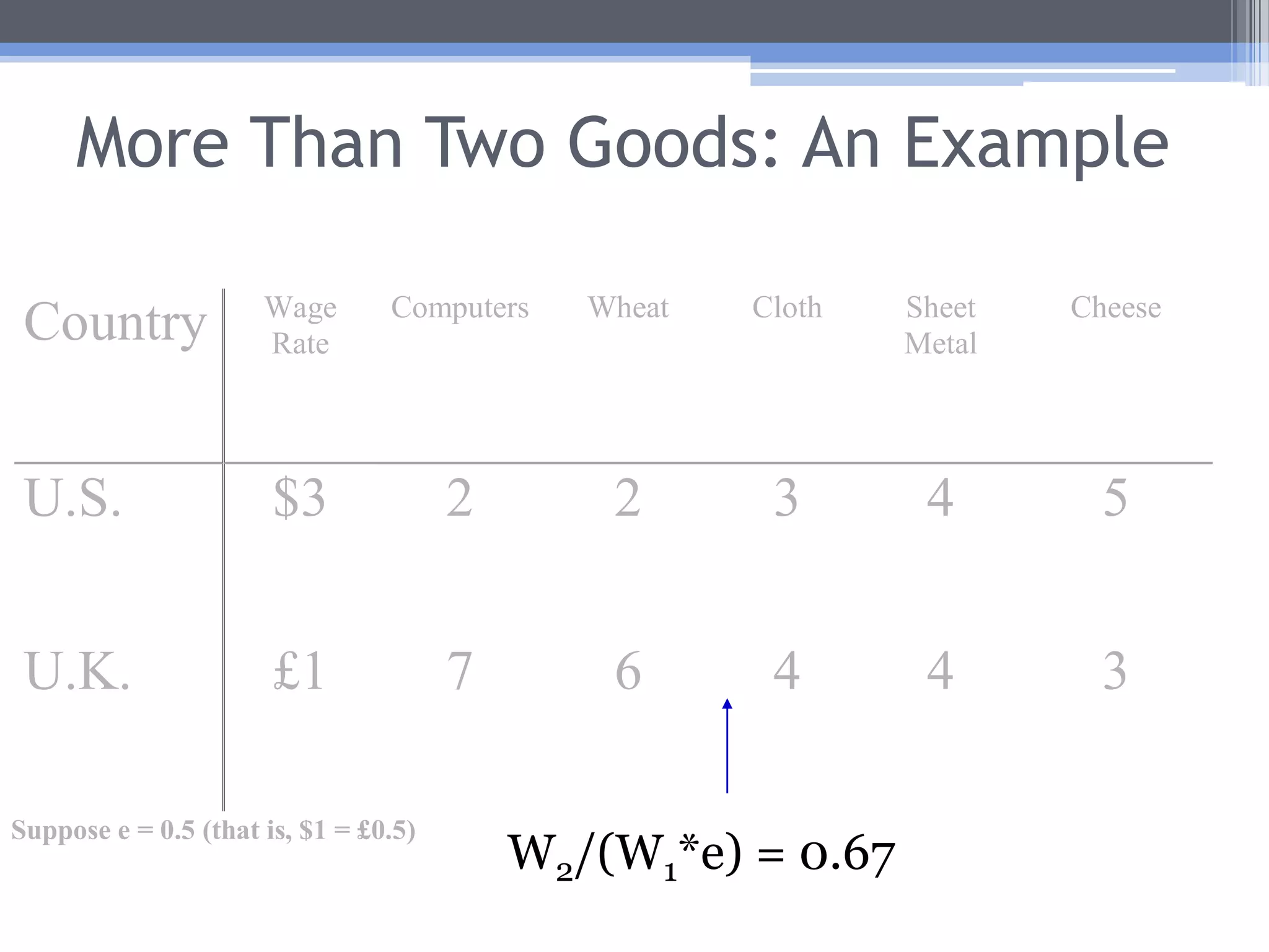
    More Than TwoGoods: An ExampleSuppose the exchange rate is still $1 = £0.5 (that is, e = 0.5).Then Use this as a “pointer”: Country 1 should export everything to the left of the pointer
  • 55.
    More Than TwoGoods: An ExampleW2/(W1*e) = 0.67
  • 56.
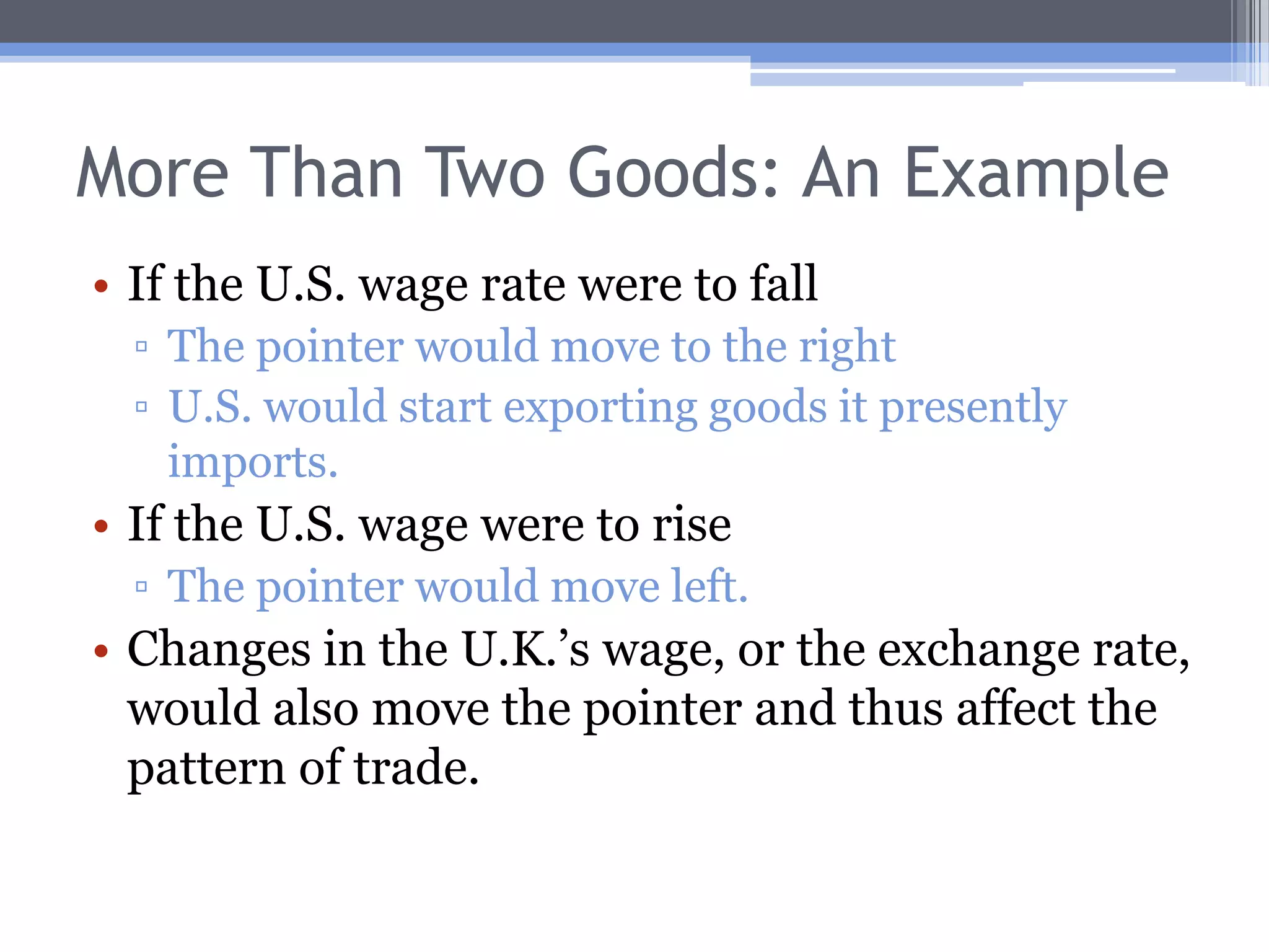
    More Than TwoGoods: An ExampleIf the U.S. wage rate were to fallThe pointer would move to the rightU.S. would start exporting goods it presently imports.If the U.S. wage were to riseThe pointer would move left.Changes in the U.K.’s wage, or the exchange rate, would also move the pointer and thus affect the pattern of trade.
  • 57.
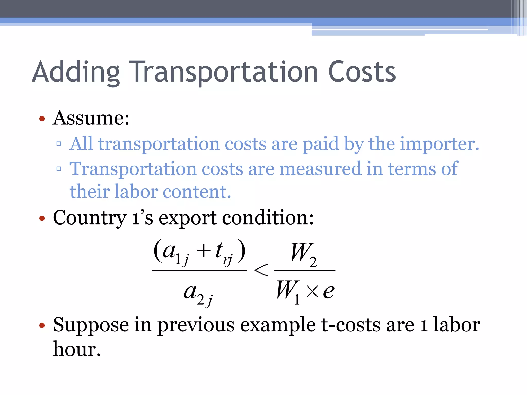
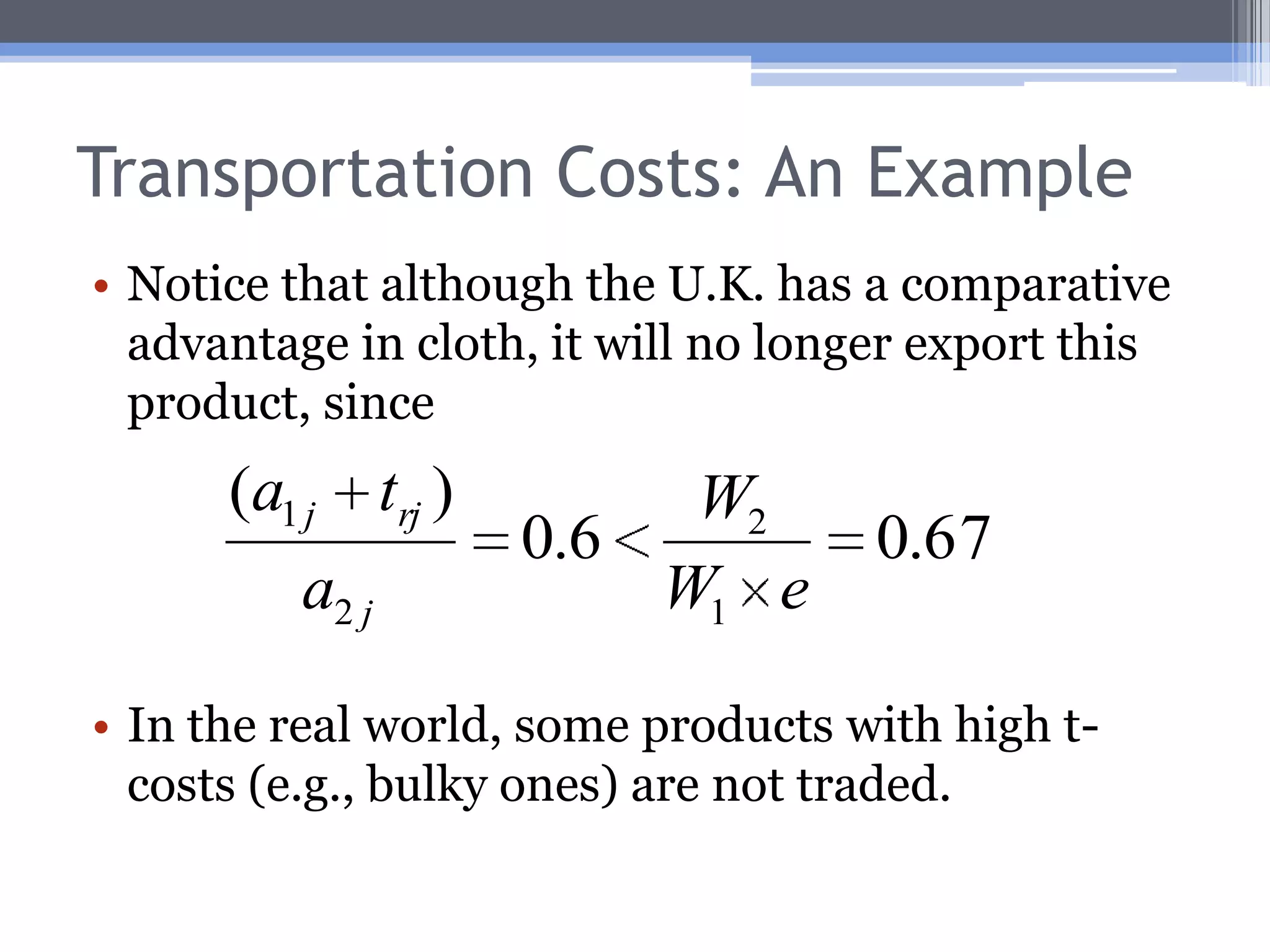
    Adding Transportation CostsAssume:Alltransportation costs are paid by the importer.Transportation costs are measured in terms of their labor content.Country 1’s export condition:Suppose in previous example t-costs are 1 labor hour.
  • 58.
    Transportation Costs: AnExampleW2/(W1*e) = 0.67
  • 59.
    Transportation Costs: AnExampleNotice that although the U.K. has a comparative advantage in cloth, it will no longer export this product, since In the real world, some products with high t-costs (e.g., bulky ones) are not traded.
  • 60.
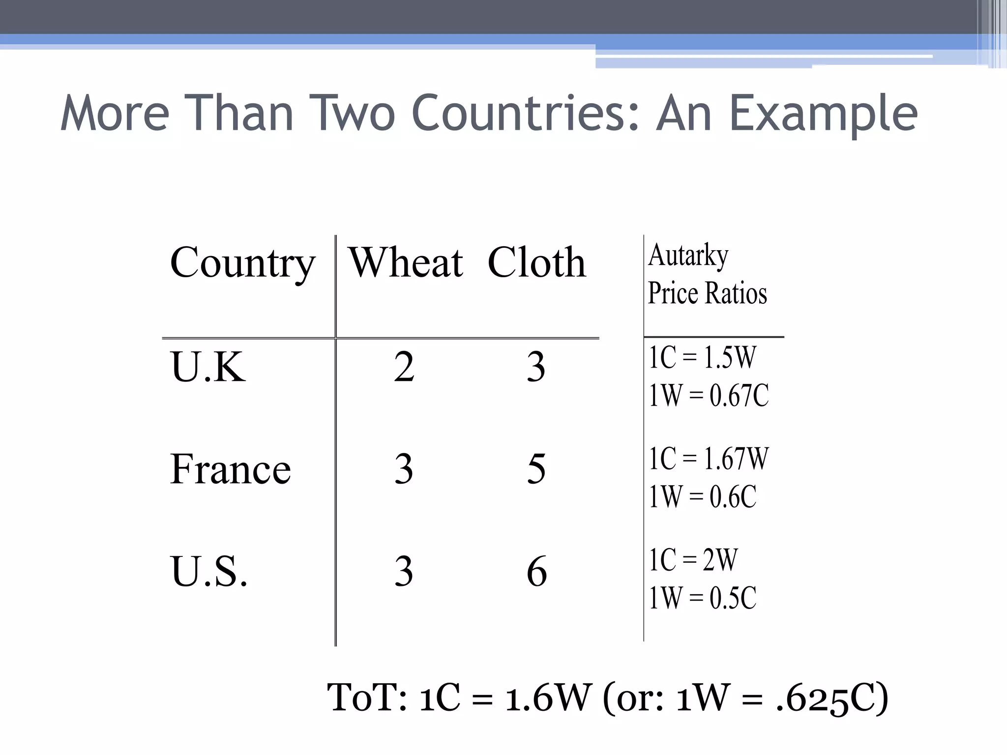
    More Than TwoCountriesHaving more than two countries also has no effect on the basic Classical model.
  • 61.
    More Than TwoCountries: An Example
  • 62.
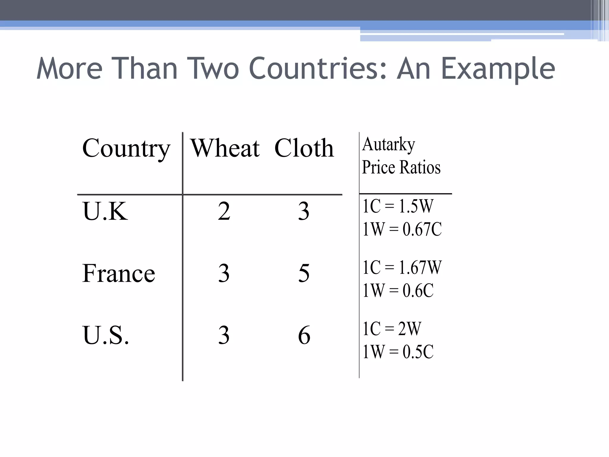
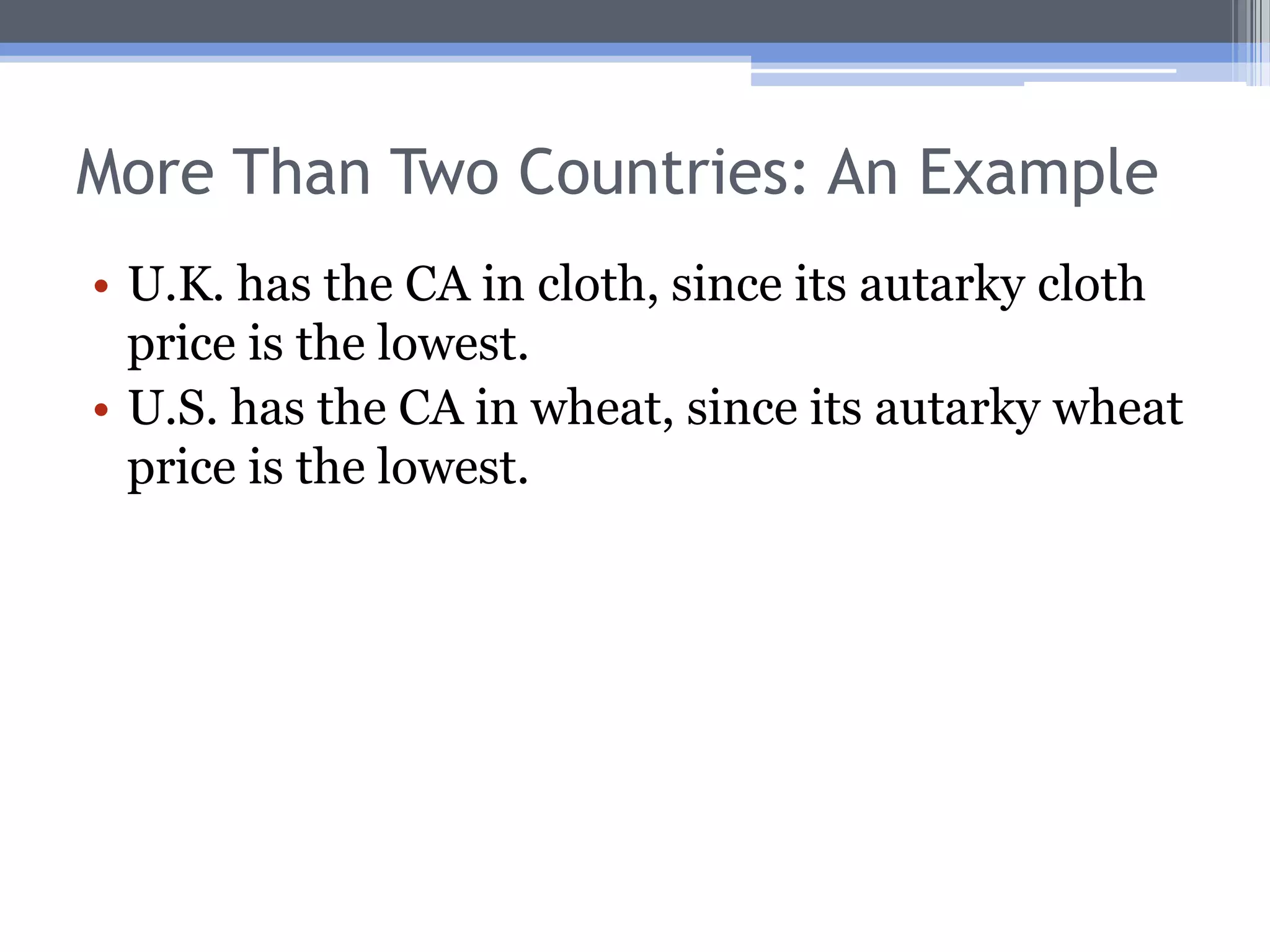
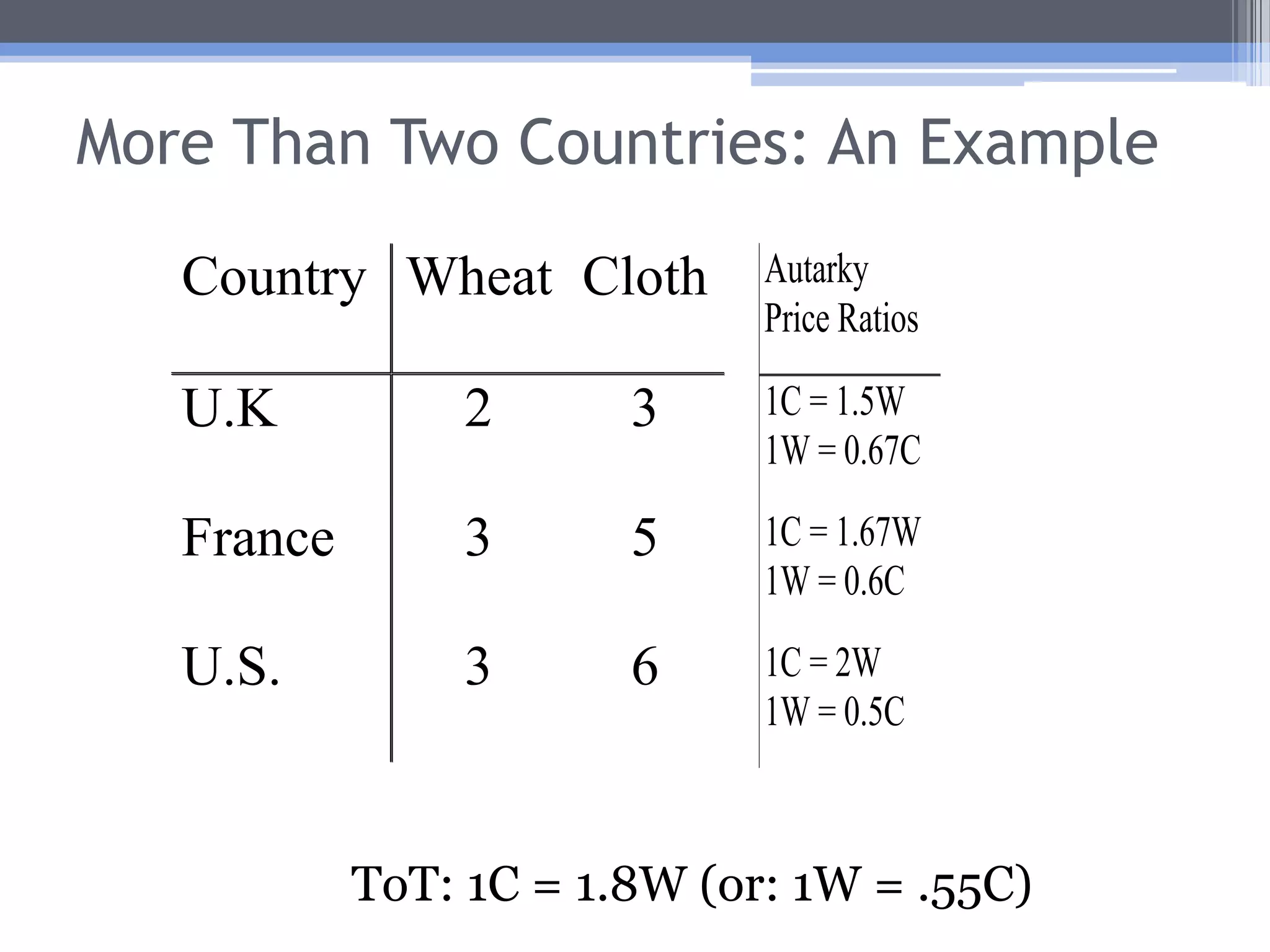
    More Than TwoCountries: An ExampleU.K. has the CA in cloth, since its autarky cloth price is the lowest.U.S. has the CA in wheat, since its autarky wheat price is the lowest.
  • 63.
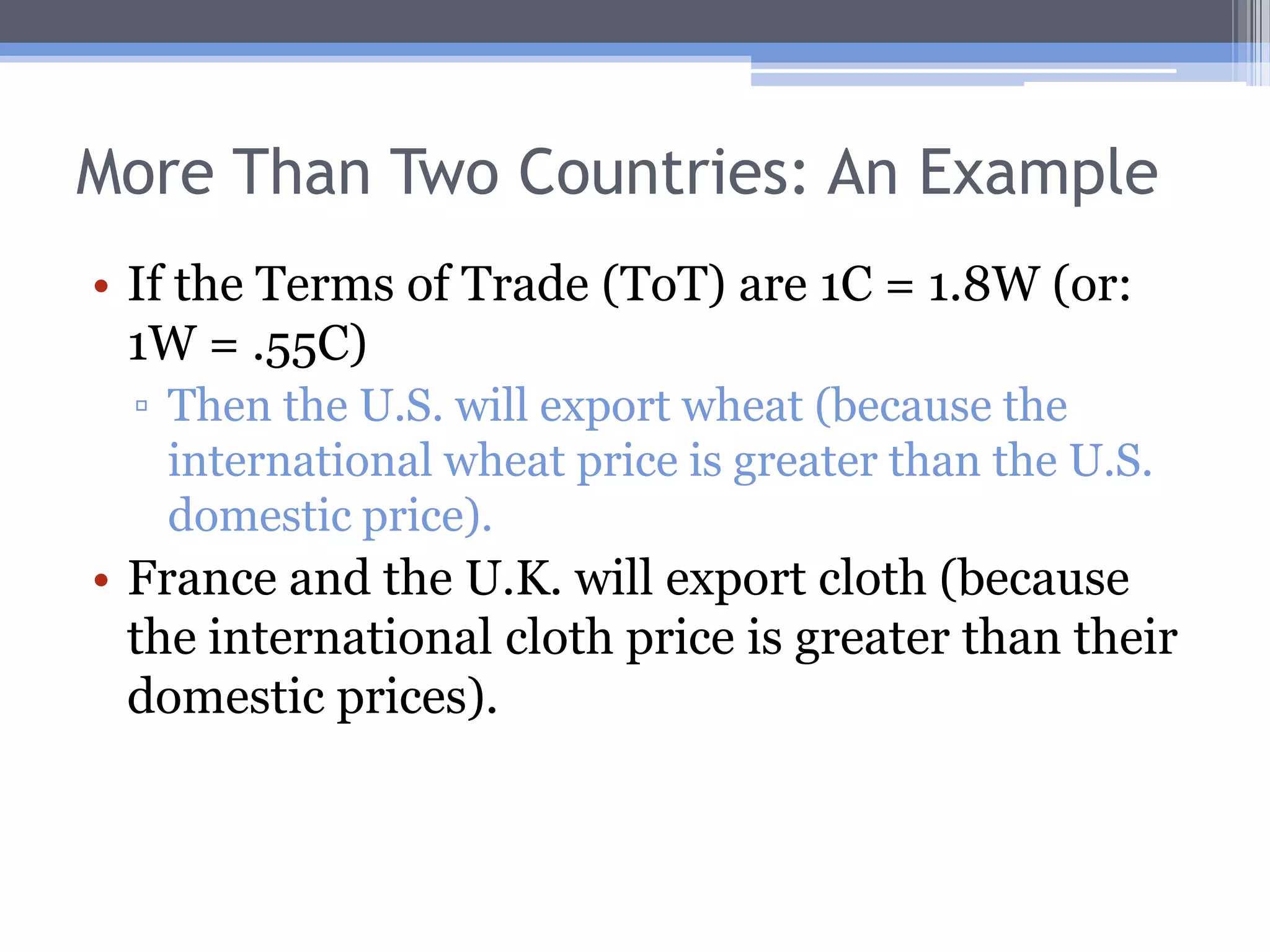
    More Than TwoCountries: An ExampleIf the Terms of Trade (ToT) are 1C = 1.8W (or: 1W = .55C)Then the U.S. will export wheat (because the international wheat price is greater than the U.S. domestic price).France and the U.K. will export cloth (because the international cloth price is greater than their domestic prices).
  • 64.
    More Than TwoCountries: An ExampleToT: 1C = 1.8W (or: 1W = .55C)
  • 65.
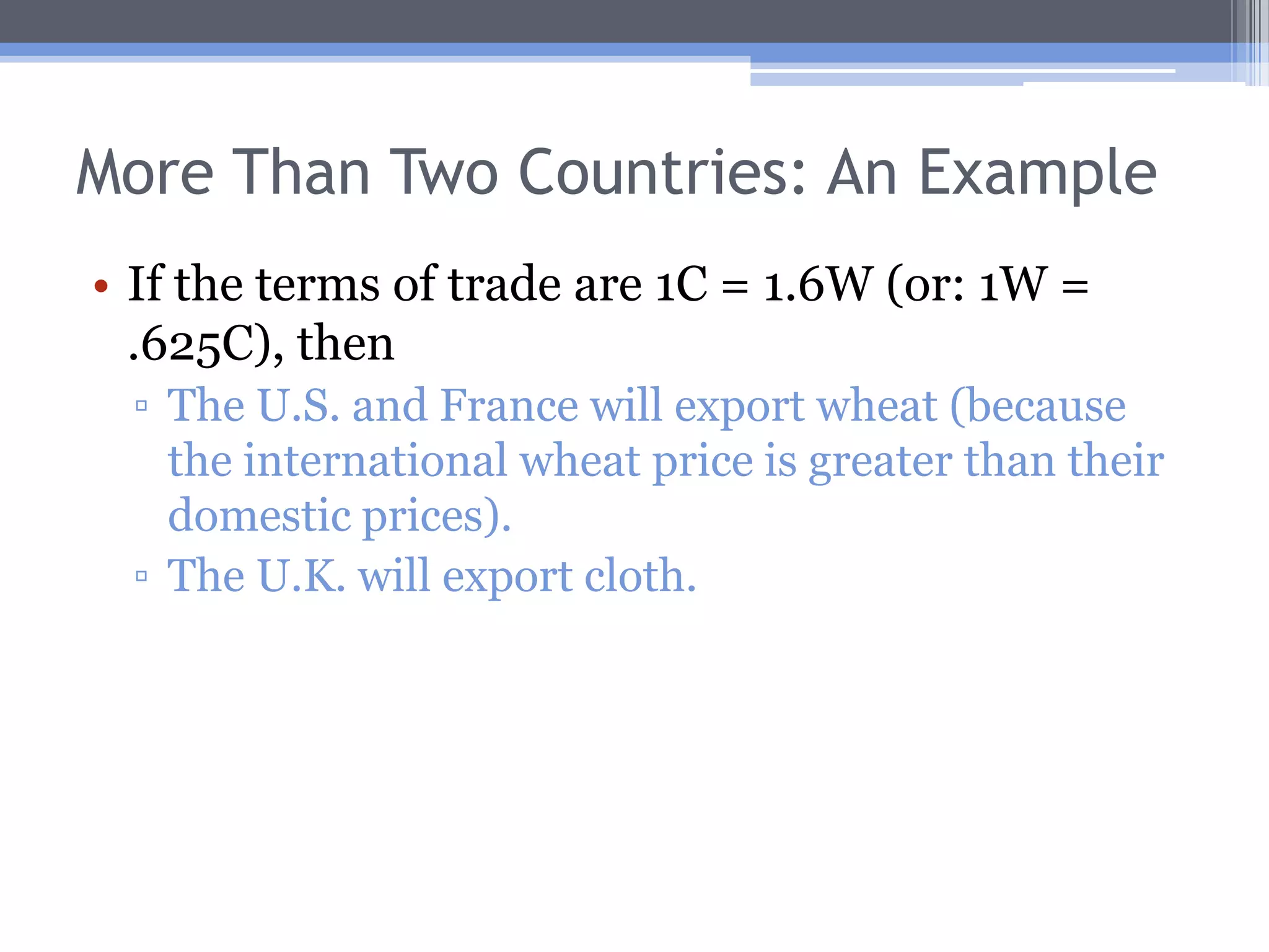
    More Than TwoCountries: An ExampleIf the terms of trade are 1C = 1.6W (or: 1W = .625C), then The U.S. and France will export wheat (because the international wheat price is greater than their domestic prices).The U.K. will export cloth.
  • 66.
    More Than TwoCountries: An ExampleToT: 1C = 1.6W (or: 1W = .625C)
  • 67.
    Evaluating the ClassicalModelEmpirical studies generally show that the classical model is consistent with observed trading patterns.However, the complexity of today’s world means the Classical model cannot supply a complete understanding of international trade.
  • 68.
    Consumer Behavior TheoryHowdo consumers decide how much of each good to consume?
  • 69.
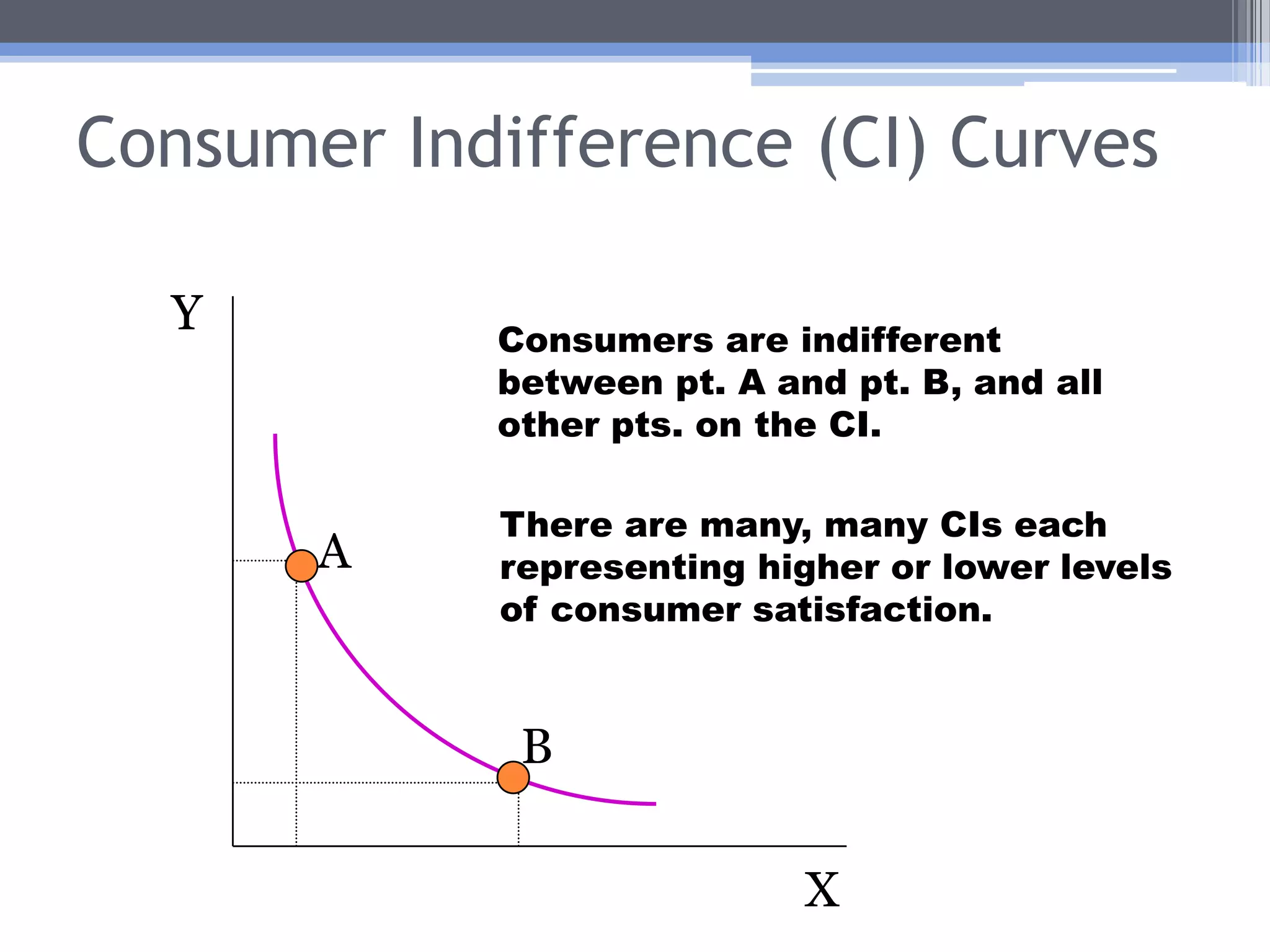
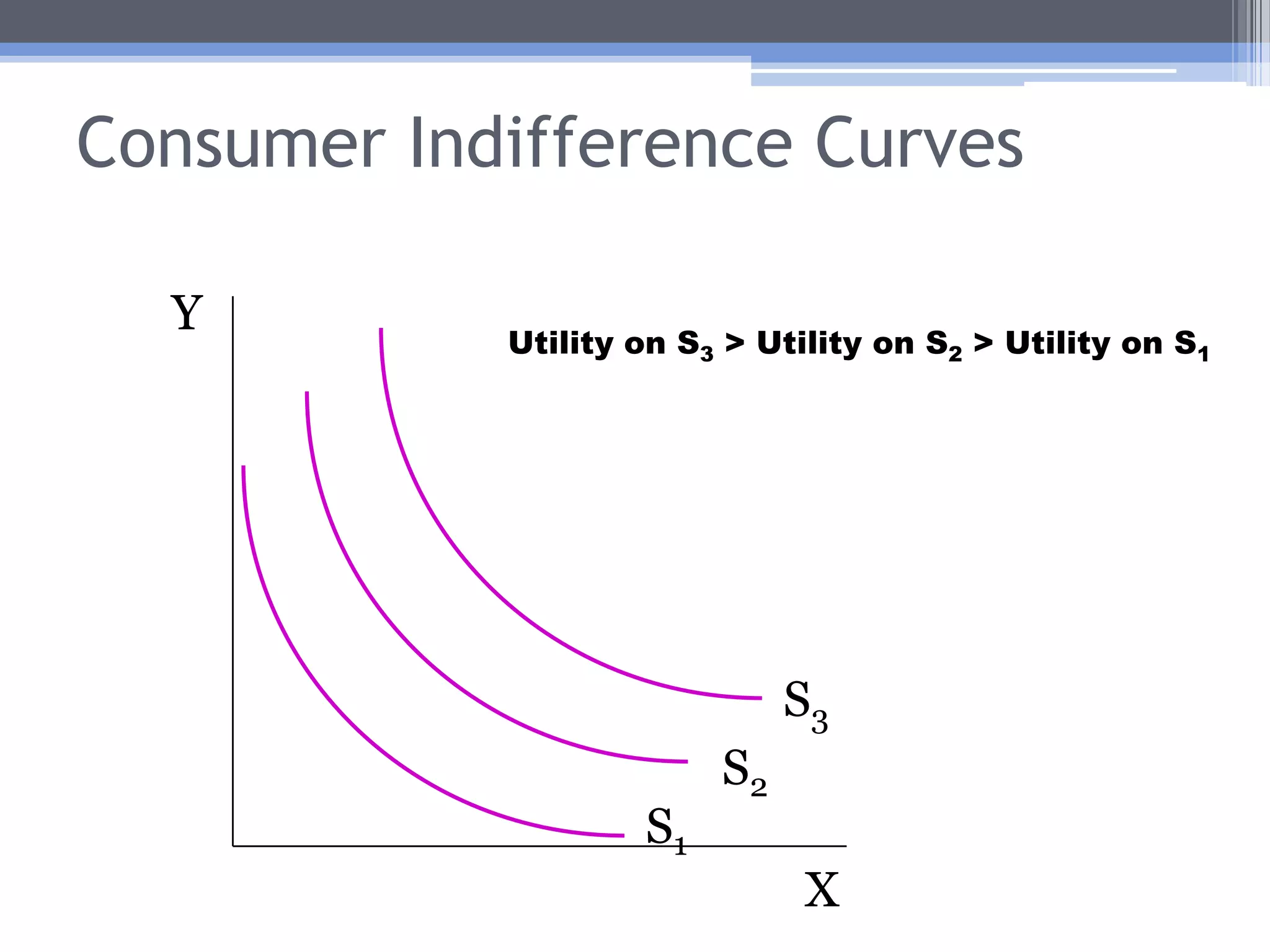
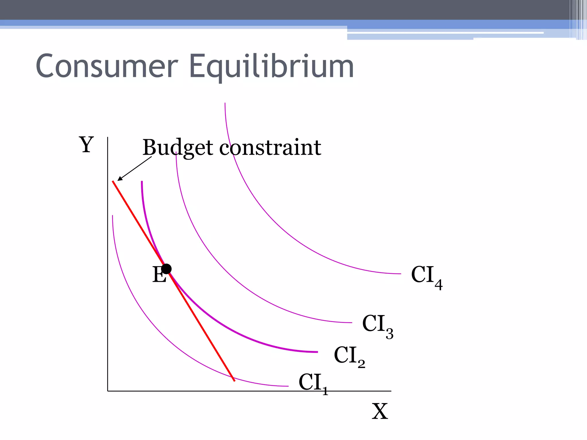
    Consumer Indifference (CI)CurvesYConsumers are indifferent between pt. A and pt. B, and all other pts. on the CI.There are many, many CIs each representing higher or lower levels of consumer satisfaction.ABX
  • 70.
    Consumer Indifference CurvesYUtilityon S3 > Utility on S2 > Utility on S1S3S2S1X
  • 71.
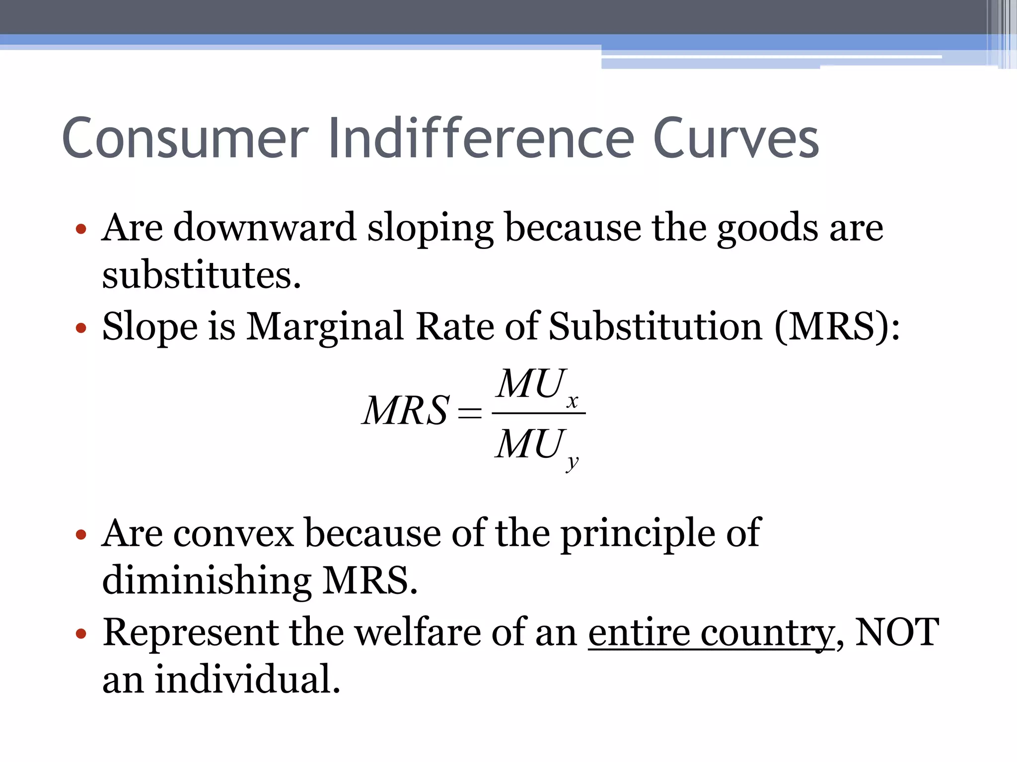
    Consumer Indifference CurvesAredownward sloping because the goods are substitutes.Slope is Marginal Rate of Substitution (MRS): Are convex because of the principle of diminishing MRS.Represent the welfare of an entire country, NOT an individual.
  • 72.
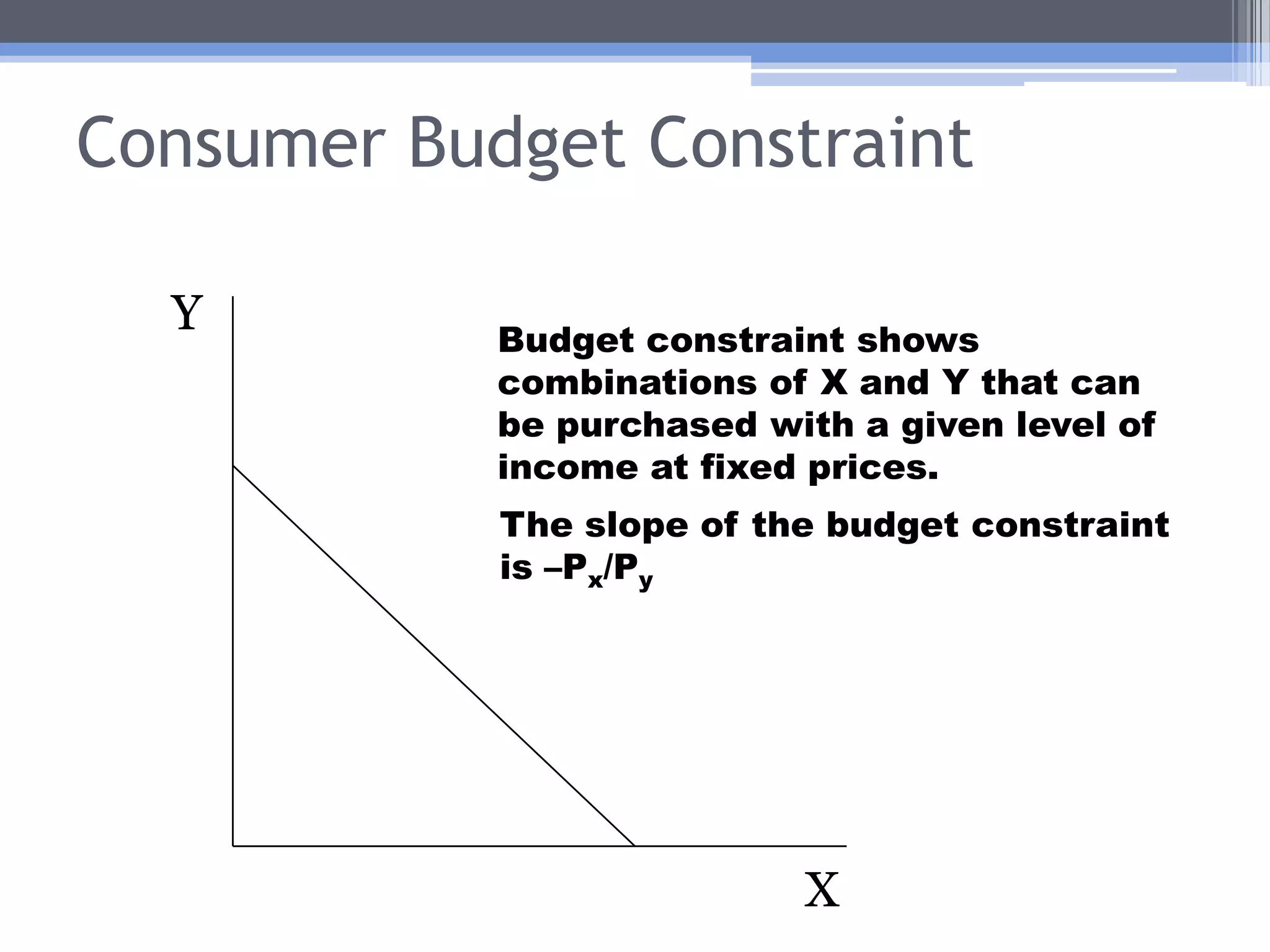
    Consumer Budget ConstraintYBudgetconstraint shows combinations of X and Y that can be purchased with a given level of income at fixed prices. The slope of the budget constraint is –Px/PyX
  • 73.
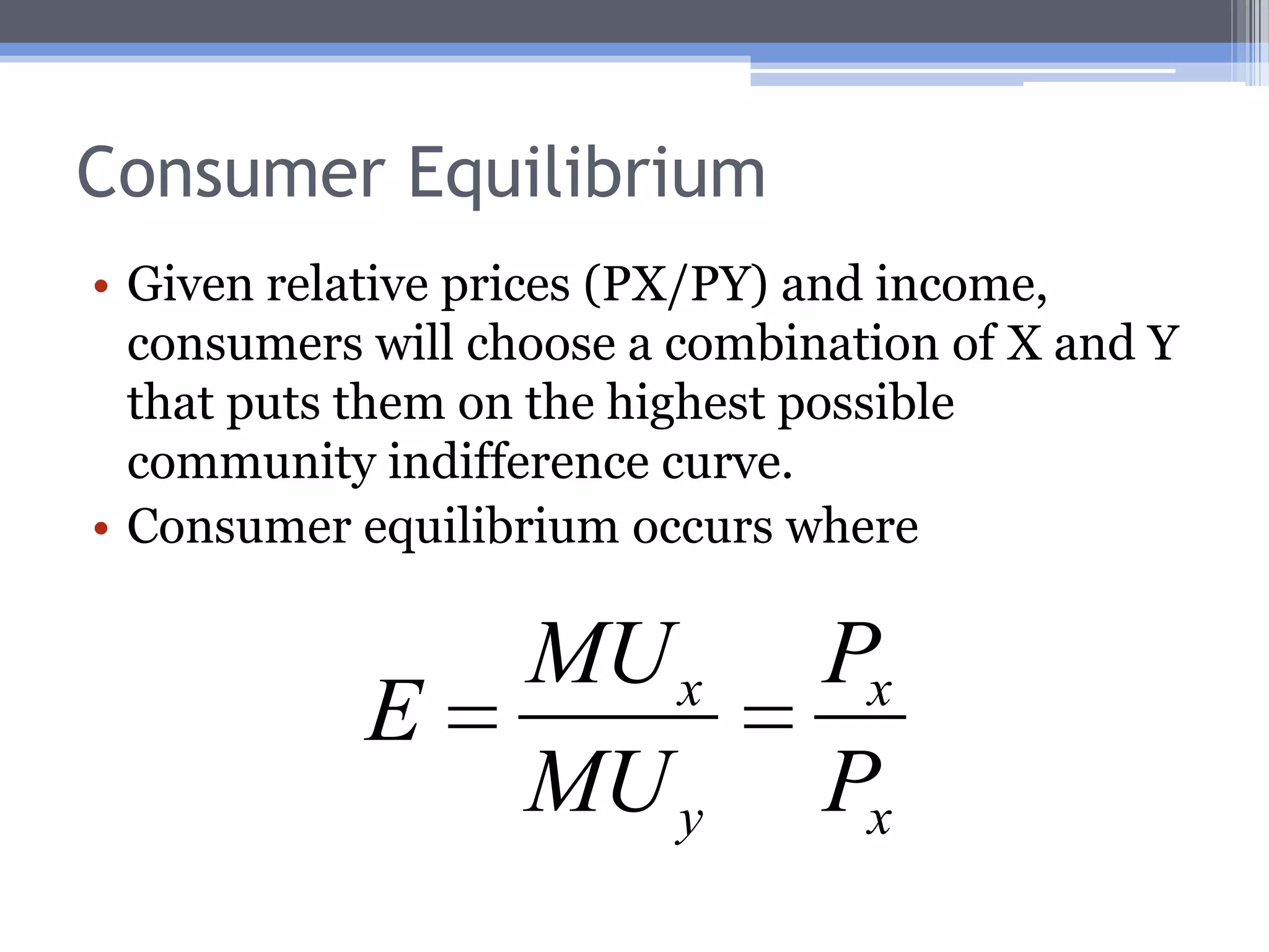
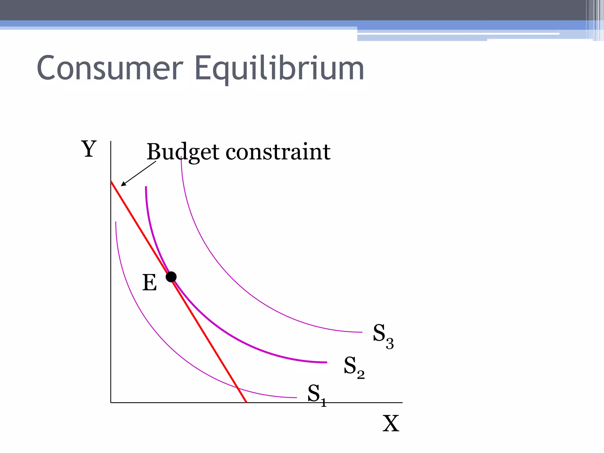
    Consumer EquilibriumGiven relativeprices (PX/PY) and income, consumers will choose a combination of X and Y that puts them on the highest possible community indifference curve.Consumer equilibrium occurs where
  • 74.
  • 75.
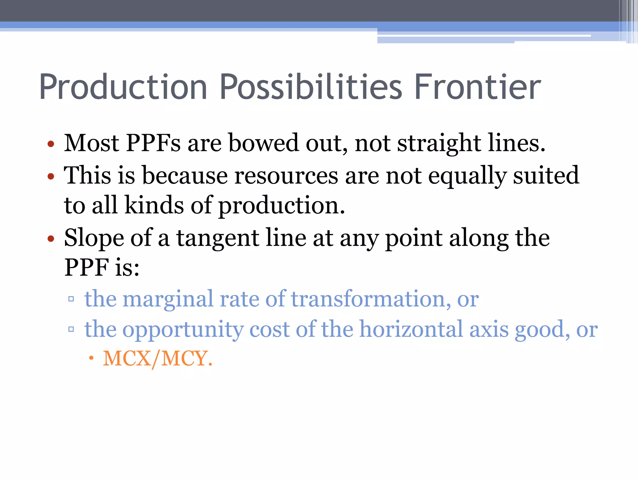
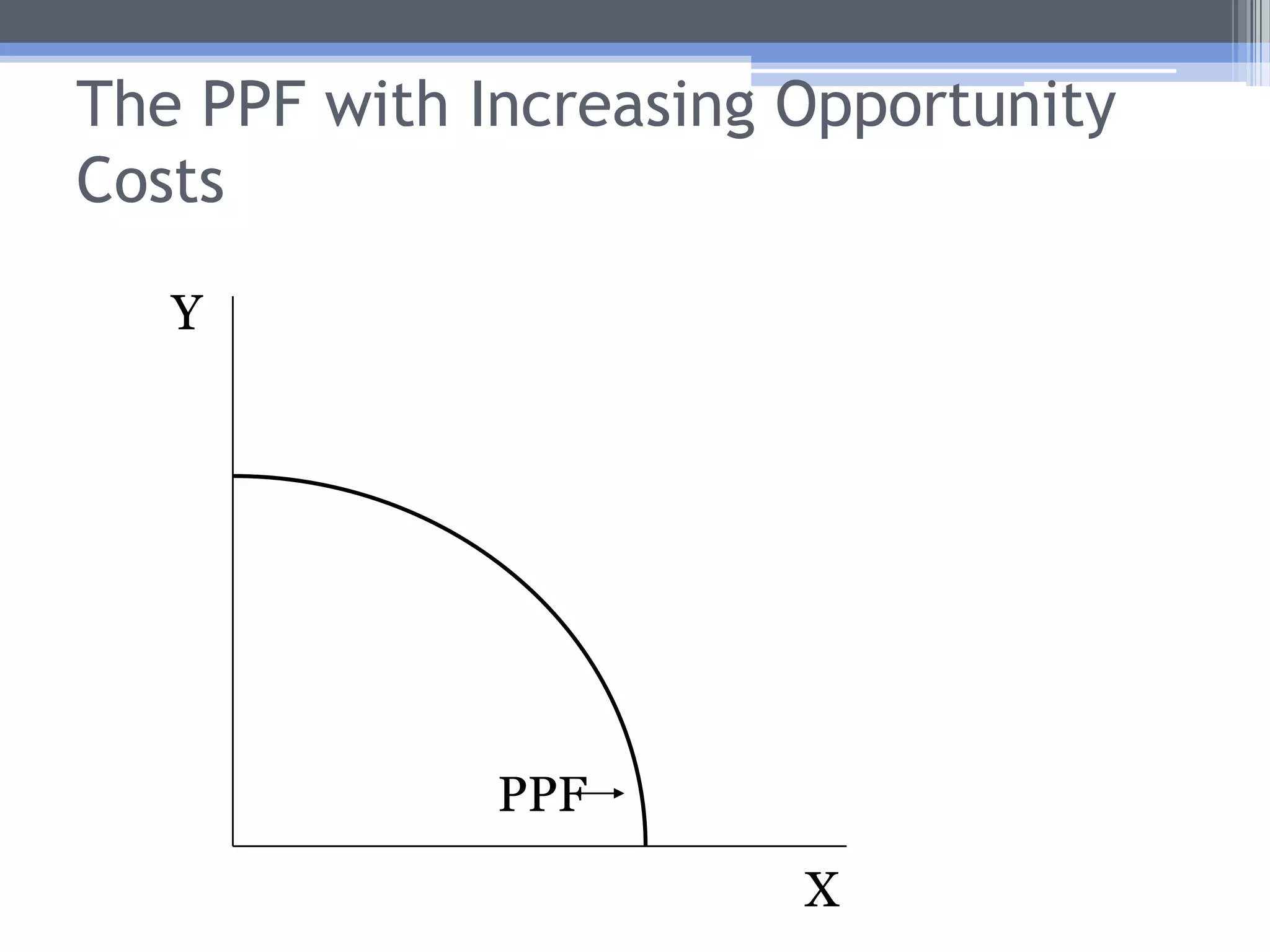
    Production Possibilities FrontierMostPPFs are bowed out, not straight lines.This is because resources are not equally suited to all kinds of production.Slope of a tangent line at any point along the PPF is:the marginal rate of transformation, orthe opportunity cost of the horizontal axis good, orMCX/MCY.
  • 76.
    The PPF withIncreasing Opportunity CostsYPPFX
  • 77.
    Problems With ClassicalTheoryLabor theory of value is unrealistic.Assumption of constant opportunity costs is too restrictive.Demand is largely ignored.
  • 78.
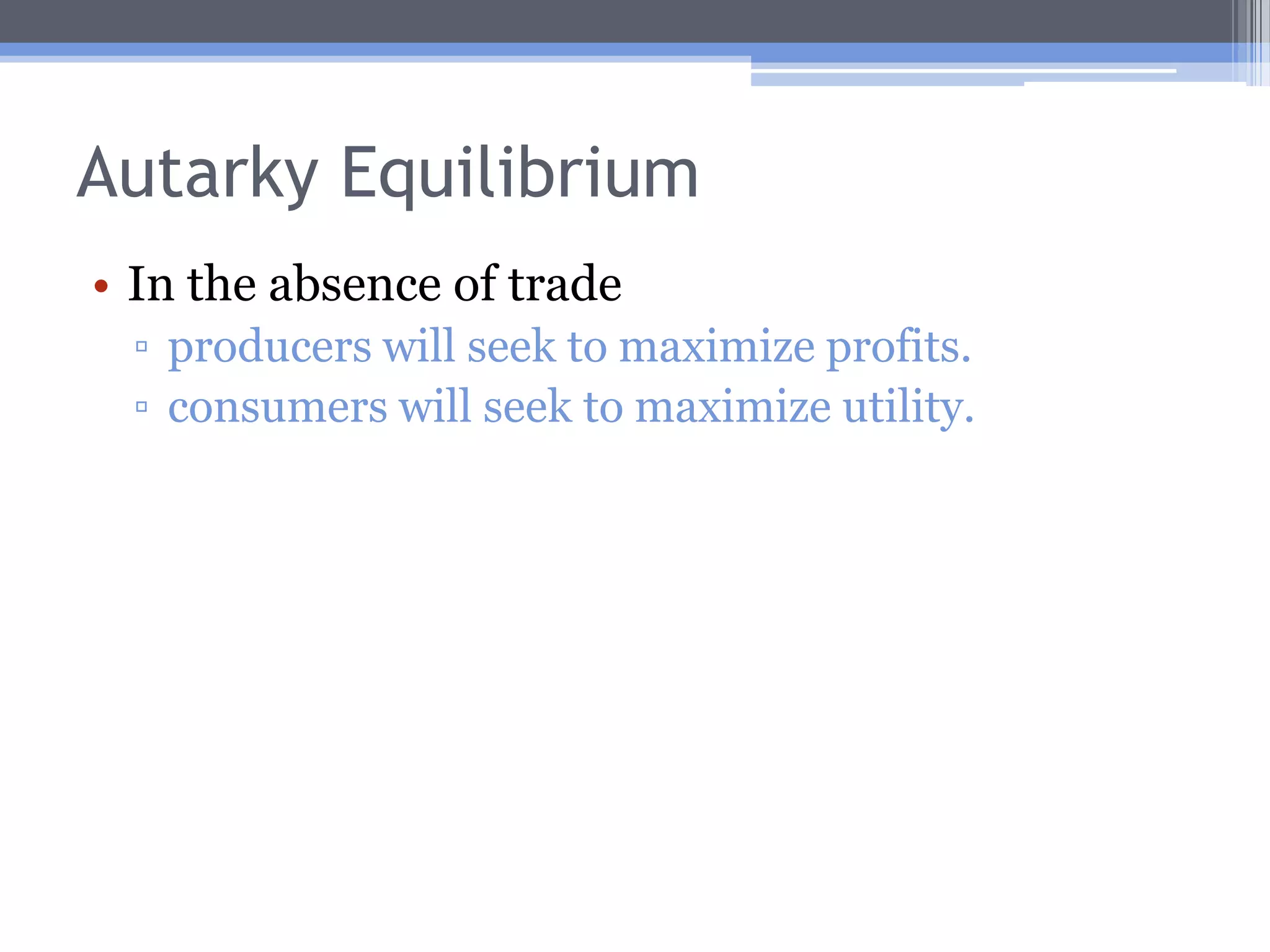
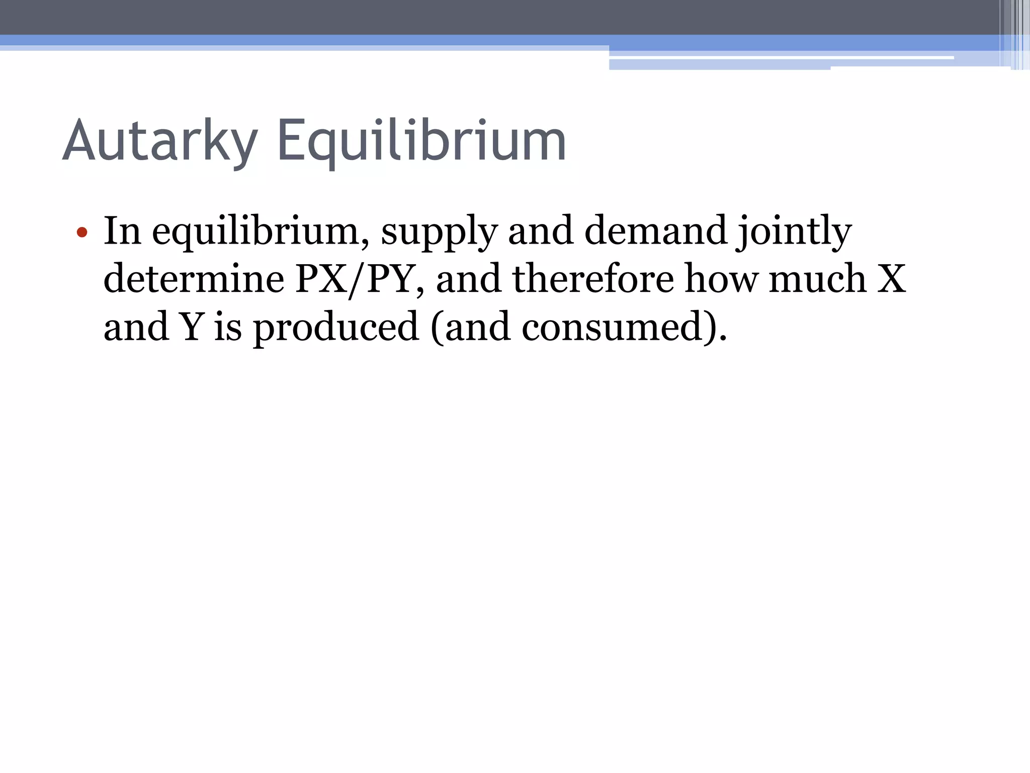
    Autarky EquilibriumIn theabsence of trade producers will seek to maximize profits.consumers will seek to maximize utility.
  • 79.
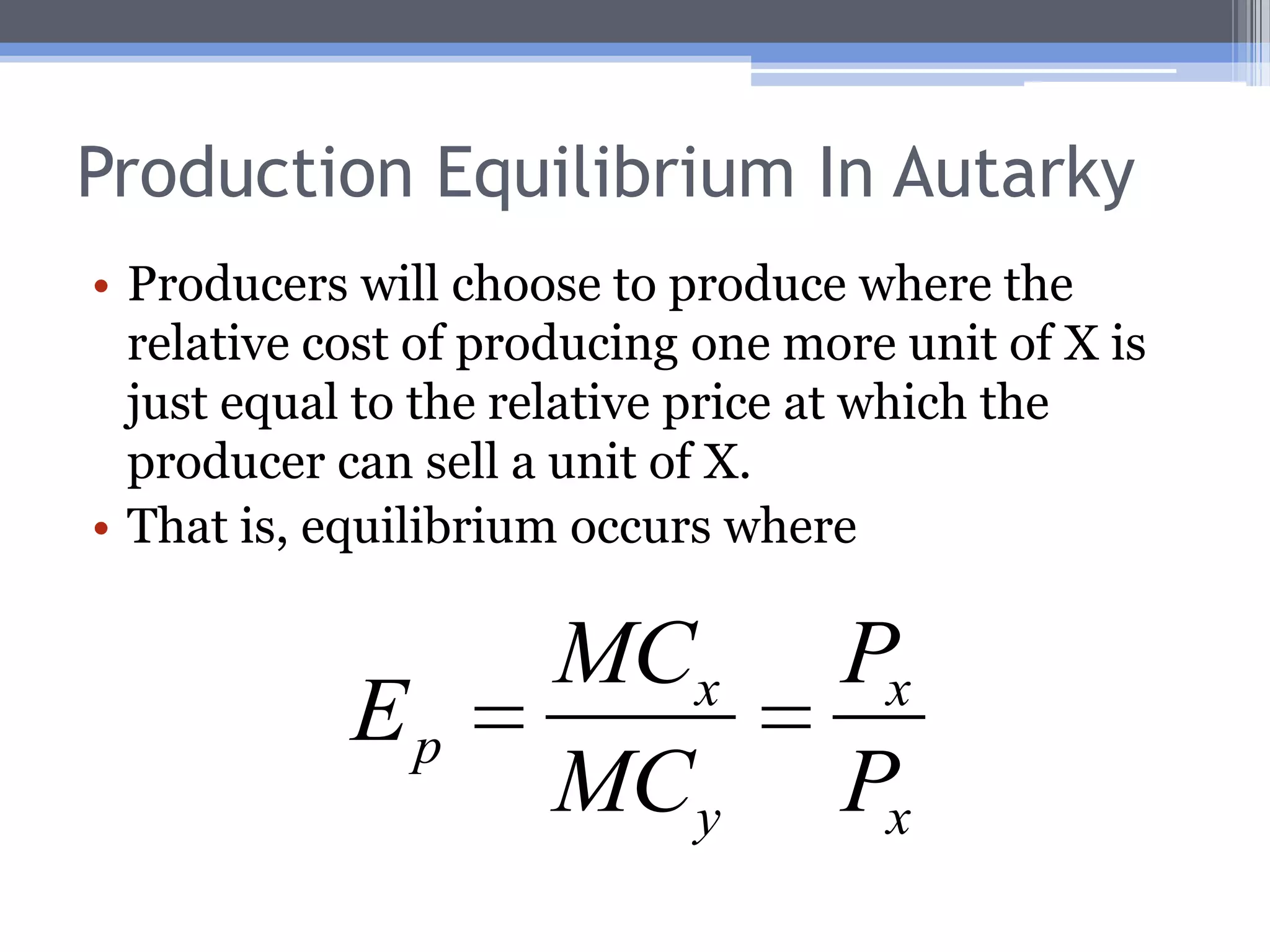
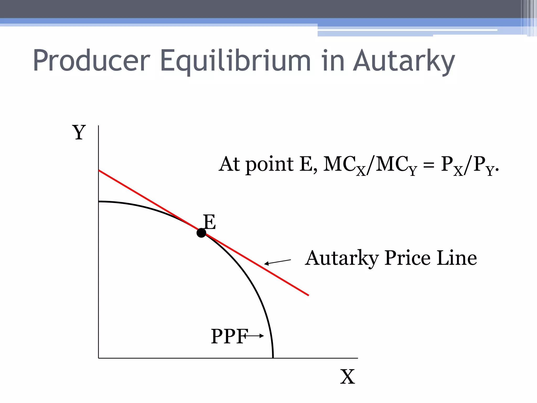
    Production Equilibrium InAutarkyProducers will choose to produce where the relative cost of producing one more unit of X is just equal to the relative price at which the producer can sell a unit of X.That is, equilibrium occurs where
  • 80.
    Producer Equilibrium inAutarkyYAt point E, MCX/MCY= PX/PY.EAutarky Price LinePPFX
  • 81.
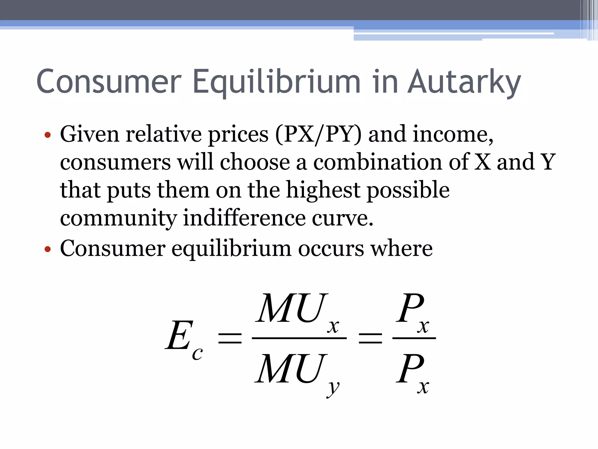
    Consumer Equilibrium inAutarkyGiven relative prices (PX/PY) and income, consumers will choose a combination of X and Y that puts them on the highest possible community indifference curve.Consumer equilibrium occurs where
  • 82.
  • 83.
    Autarky EquilibriumIn equilibrium,supply and demand jointly determine PX/PY, and therefore how much X and Y is produced (and consumed).
  • 84.
  • 85.
    The Introduction ofInternational TradeTrade will cause relative prices to change.Producers will respond to this by altering relative production of goods X and Y.Consumers will respond to this by altering relative consumption of goods X and Y.
  • 86.
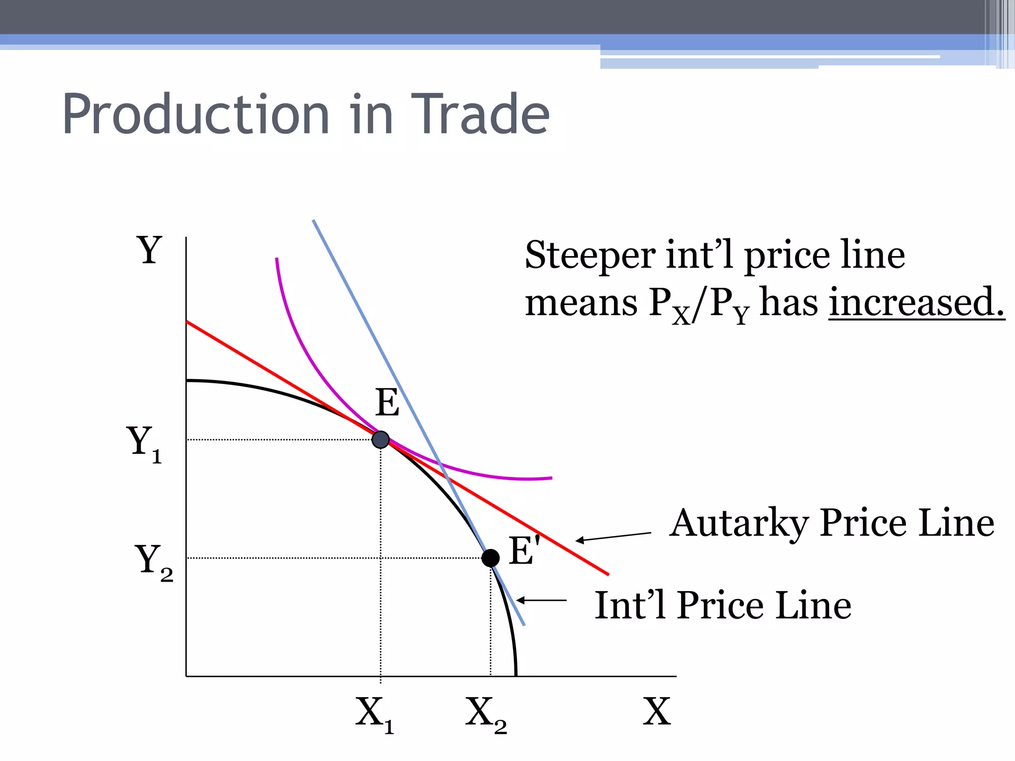
    Production in TradeLet’ssuppose that Country A has a comparative advantage in good X.What will happen to the relative price of good X as Country A moves to trade?It will rise (otherwise, Country A would not wish to produce more of good X in order to export it).
  • 87.
    Production in TradeYSteeperint’l price linemeans PX/PY has increased.EY1Autarky Price LineE'Y2Int’l Price LineXX1X2
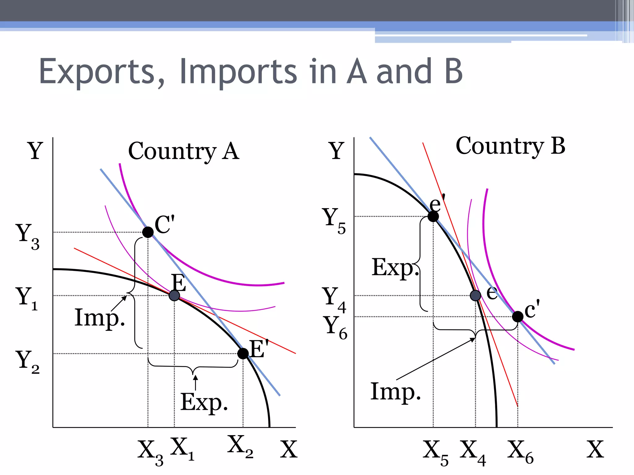
  • 88.
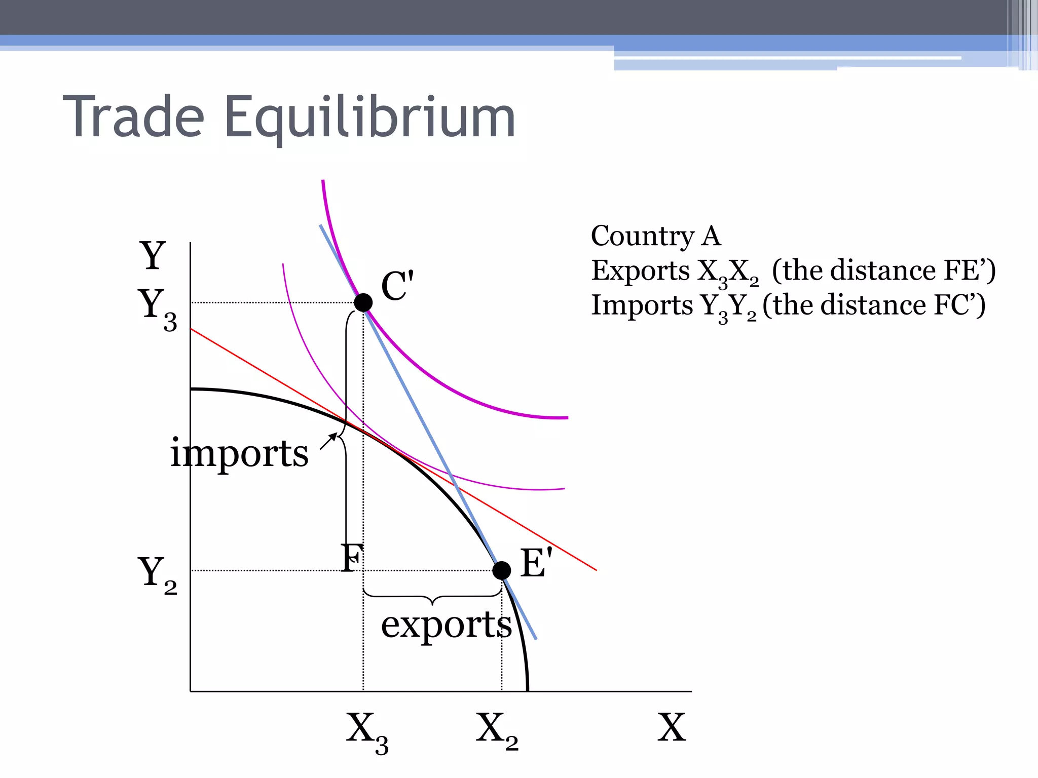
    Trade EquilibriumCountry AExports X3X2 (the distance FE’)Imports Y3Y2 (the distance FC’)YC'Y3importsFE'Y2exportsXX2X3
  • 89.
    Movement From Autarkyto TradeMovement to trade causes relative price of good X to rise.Higher relative price means more X will be produced, less Y .Higher relative price of X lowers consumption of X, raises consumption of Y.Extra X is exported, shortfall in Y is met by imports.
  • 90.
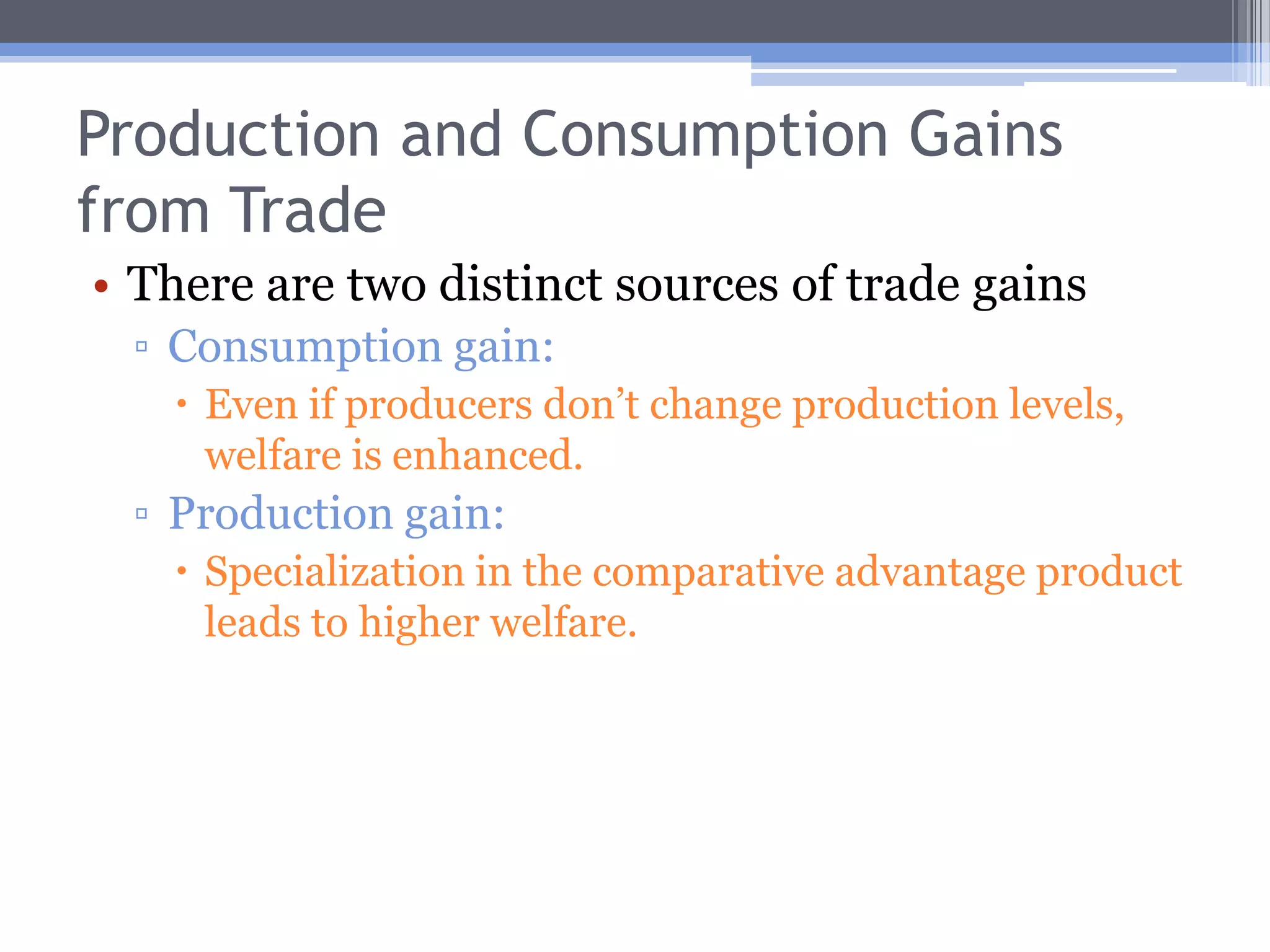
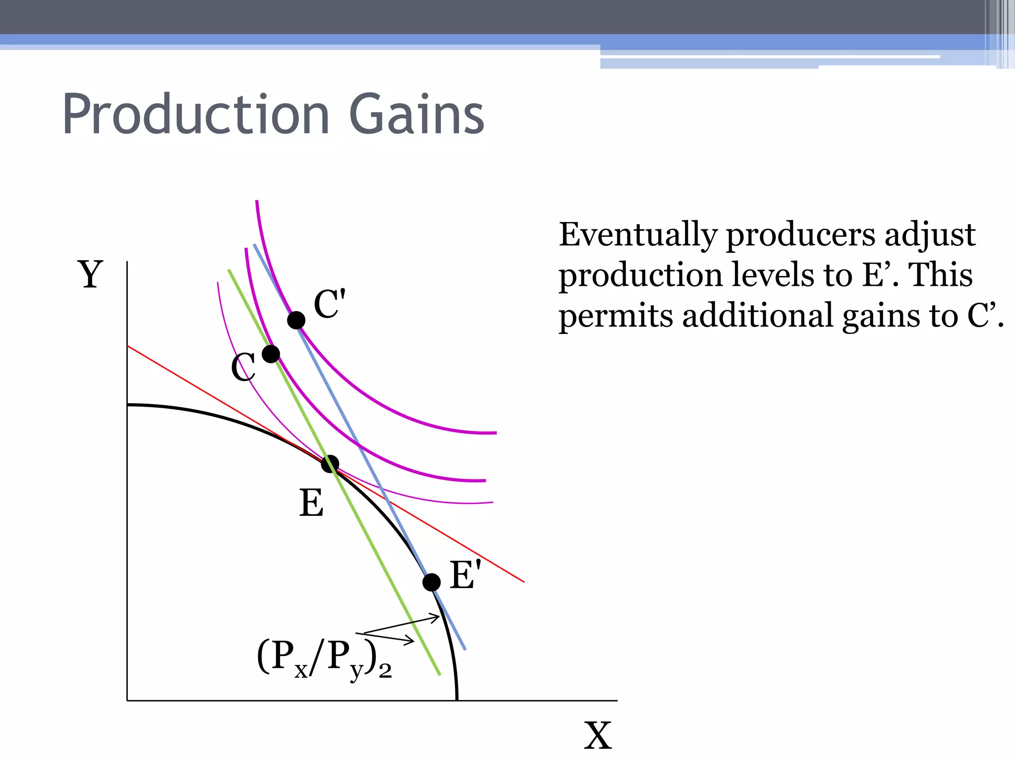
    Production and ConsumptionGains from TradeThere are two distinct sources of trade gainsConsumption gain: Even if producers don’t change production levels, welfare is enhanced.Production gain: Specialization in the comparative advantage product leads to higher welfare.
  • 91.
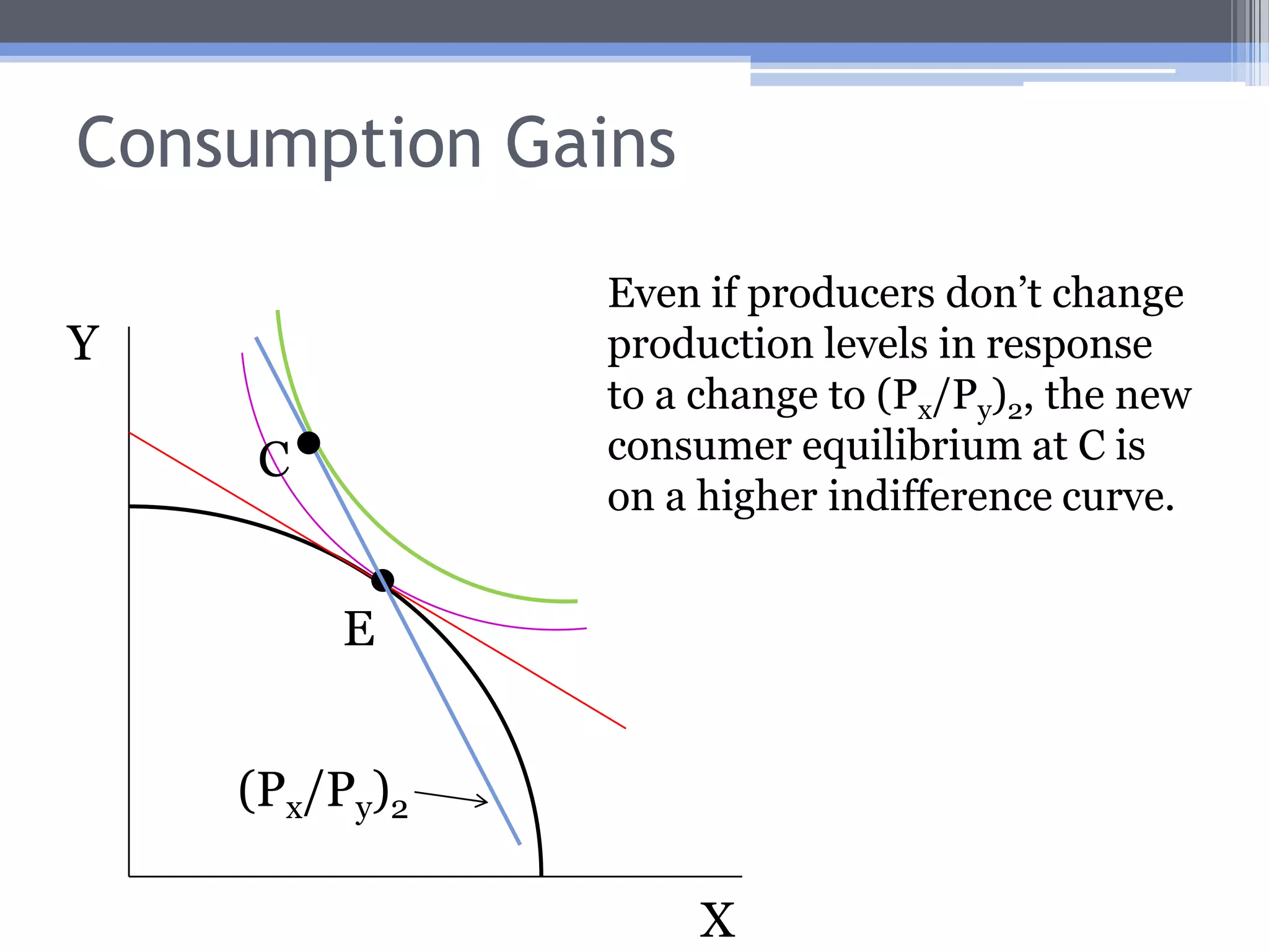
    Consumption GainsEven ifproducers don’t change production levels in response to a change to (Px/Py)2, the new consumer equilibrium at C is on a higher indifference curve.YCE(Px/Py)2X
  • 92.
    Production GainsEventually producersadjust production levels to E’. This permits additional gains to C’.YC'CEE'(Px/Py)2X
  • 93.
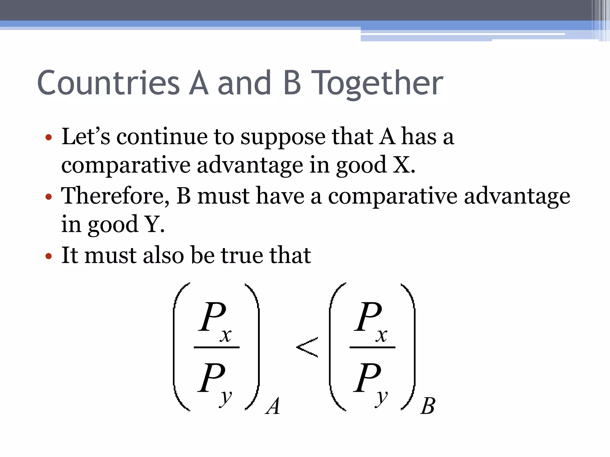
    Countries A andB TogetherLet’s continue to suppose that A has a comparative advantage in good X.Therefore, B must have a comparative advantage in good Y.It must also be true that
  • 94.
    Exports, Imports inA and BCountry BCountry AYYe'Y5C'Y3Exp.EeY1Y4c'Imp.Y6E'Y2Imp.Exp.X2X1XXX4X5X3X6
  • 95.
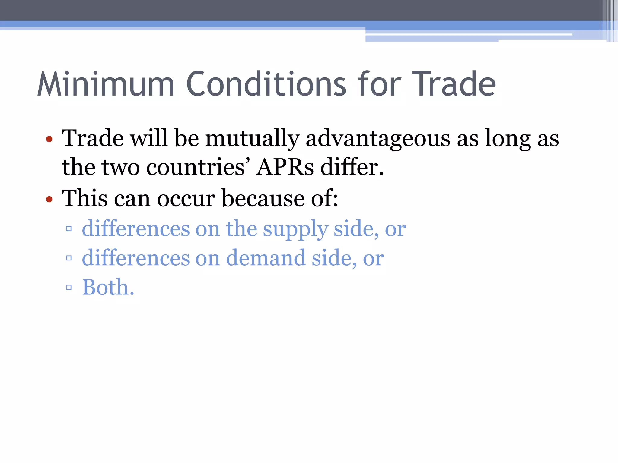
    Minimum Conditions forTradeTrade will be mutually advantageous as long as the two countries’ APRs differ.This can occur because of:differences on the supply side, ordifferences on demand side, orBoth.
  • 96.
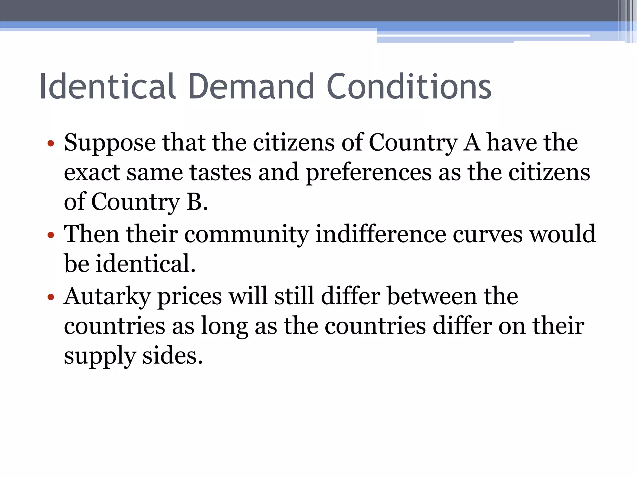
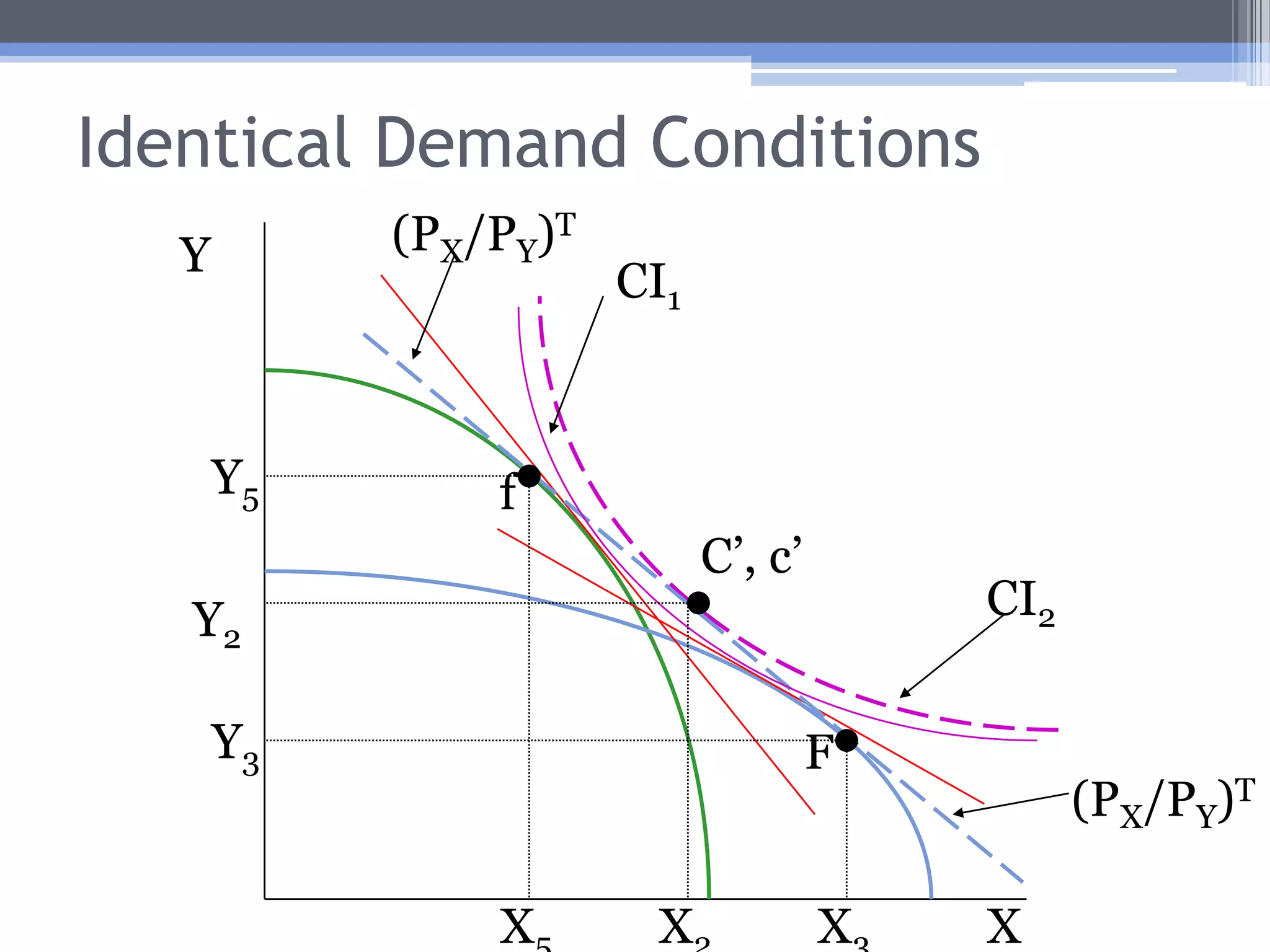
    Identical Demand ConditionsSupposethat the citizens of Country A have the exact same tastes and preferences as the citizens of Country B.Then their community indifference curves would be identical.Autarky prices will still differ between the countries as long as the countries differ on their supply sides.
  • 97.
  • 98.
    Identical Demand ConditionsEvenif demand conditions are the same, differences in supply conditions would cause differences in APRs across countries, and so:Trade could still be mutually advantageous.Implicitly, this is what is going on in the Classical model.
  • 99.
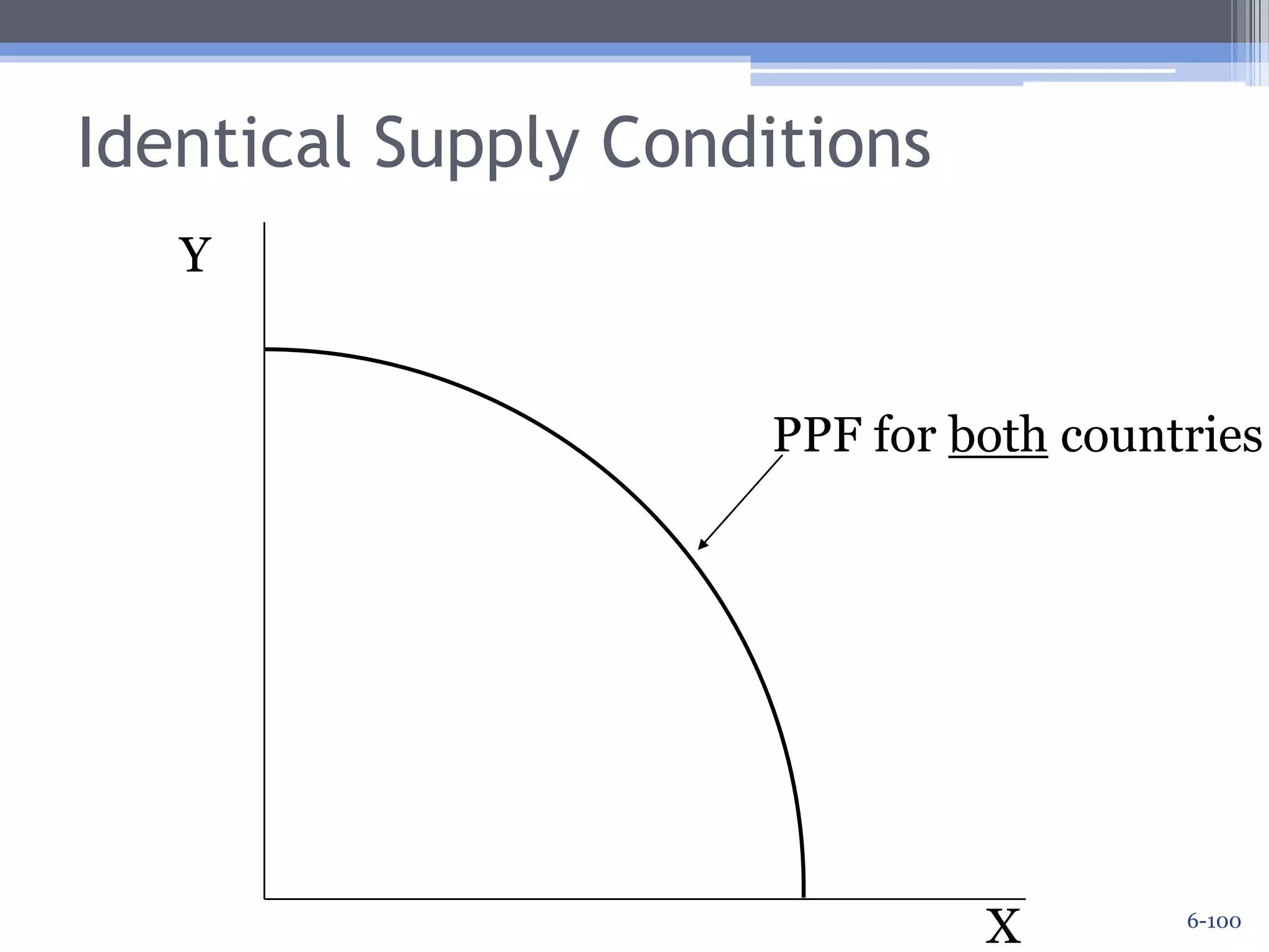
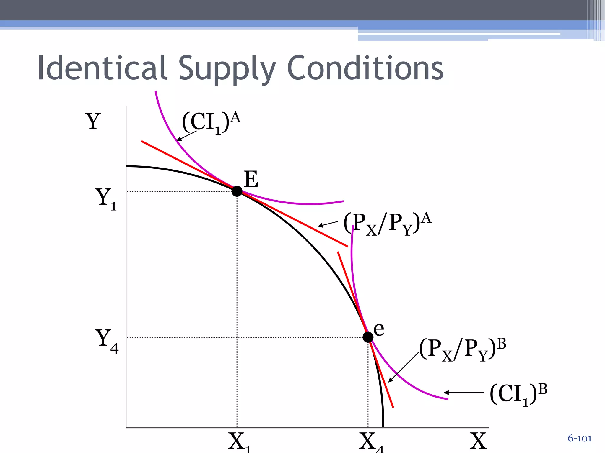
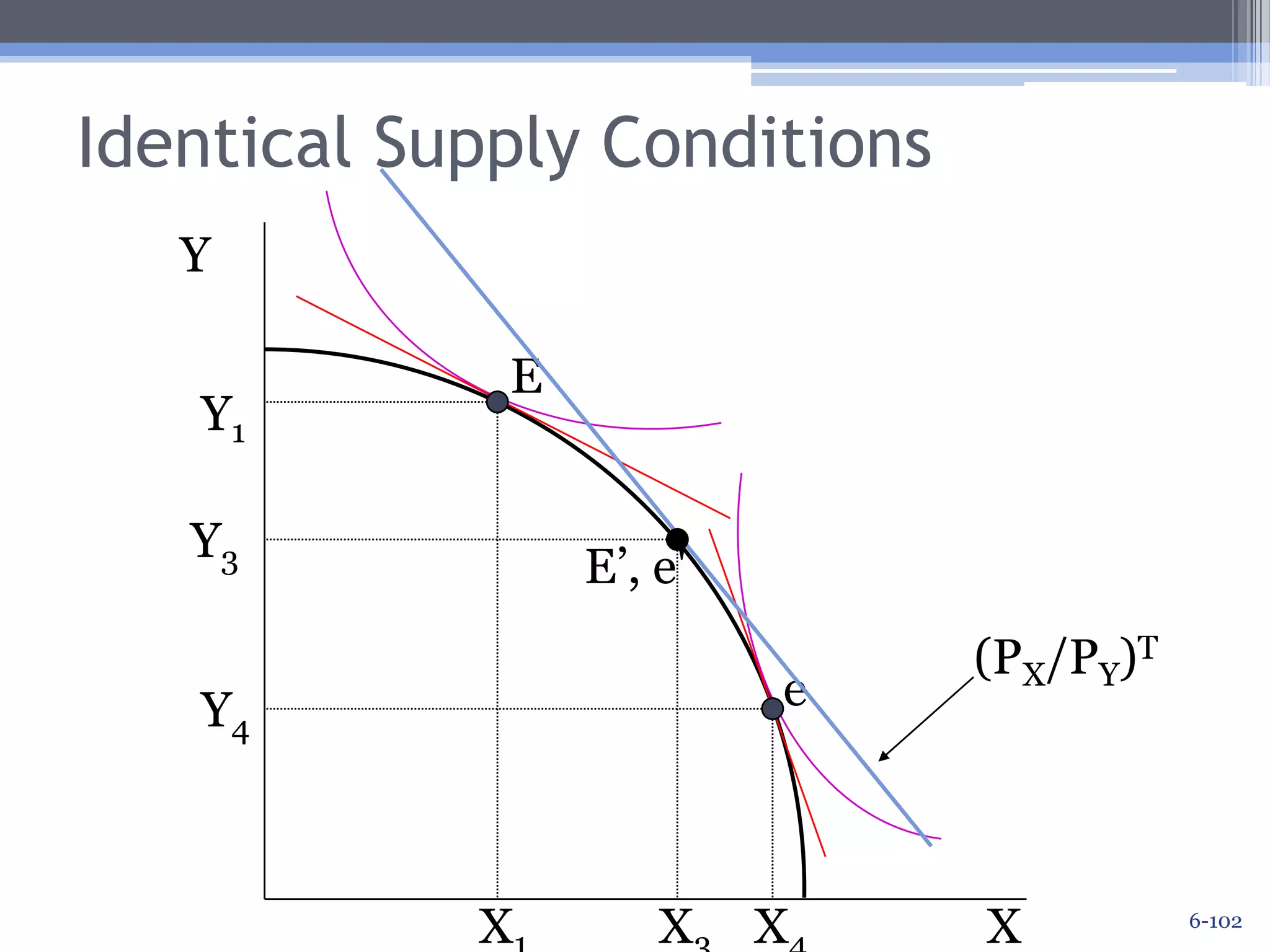
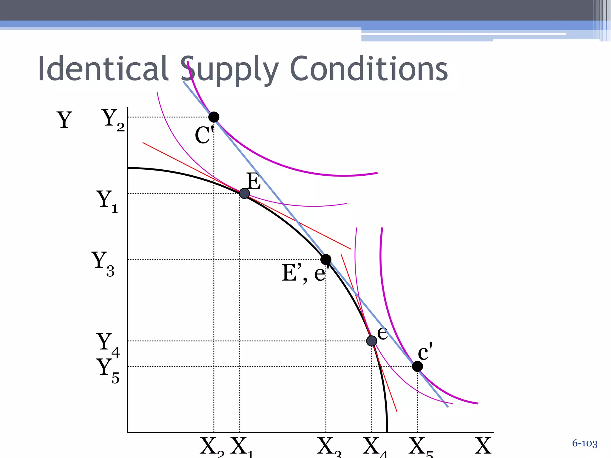
    Identical Supply ConditionsWhatif two countries have identical technologies and resource endowments?Then their PPFs would be identical.The Classical model would predict no trade, but what does the Neoclassical model show?
  • 100.
    Identical Supply ConditionsYPPFfor both countriesX6-100
  • 101.
  • 102.
  • 103.
  • 104.
    Identical Supply ConditionsEvenif supply conditions are the same, differences in demand conditions would cause differences in APRs across countries, and so:Trade could still be mutually advantageous.This was not a possibility in the Classical model, because it assumed away demand.
  • 105.
    Offer Curvescomprise allcombinations of a country’s desired exports and imports at different terms of trade.are also known as reciprocal demand curves (J.S. Mill).measure a country’s willingness to trade.can be derived from the PPF-indifference curve graph.
  • 106.
  • 107.
  • 108.
  • 109.
    Offer CurvesOffer curvesrepresent willingness to trade at every possible terms of trade.As the relative price of good X rises, Country A becomes willing to export more and import more.Offer curves “bow” towards the import good axis.
  • 110.
    Deriving Country B’sOffer CurveThis will reflect Country B’s willingness to trade at different terms of trade.B’s offer curve bows towards the axis with B’s import good on it.
  • 111.
  • 112.
  • 113.
    Terms of TradeEquilibriumThe international terms of trade (that is, PX/PY) will be the slope of a line passing through the point where the offer curves cross.This equilibrium point takes into account demand and supply conditions in both countries.
  • 114.
    Terms of TradeEquilibriumOCA(PX/PY)EYOCBY1If these are the terms of trade,country A will desire to exportX1 units, and country B will want to import X1 units.X1X
  • 115.
    Terms of TradeEquilibriumOCA(PX/PY)EYOCBY1If these are the terms of trade,country A will desire to importY1 units, and country B will want to export Y1 units. X1X
  • 116.
    How Do WeKnow It’s Equilibrium?Any terms of trade other than (PX/PY)E will result inexcess demand for one good, andexcess supply for the other.Therefore relative prices will adjust until (PX/PY)E is reached.
  • 117.
  • 118.
    DisequilibriumOCA(PX/PY)1YY1OCBY2At (PX/PY)1, countryA wishesto import Y1 units, but country B is only interested in exporting Y2units. That is, there is an excess demand for good Y.X
  • 119.
    DisequilibriumOCA(PX/PY)1YOCBAt (PX/PY)1, countryA wishesto export X1 units, but country B is only interested in importing X2units. That is, there is an excess supply of good X.X2X1X
  • 120.
    DisequilibriumExcess demand forY causes PY to rise.Excess supply of X causes PX to fall.Thus, (PX/PY) falls.In other words, the terms of trade line gets flatter, moving the countries in the direction of equilibrium.
  • 121.
  • 122.
    DisequilibriumTerms of tradelines that are flatter than (PX/PY)E, such as
  • 123.
  • 124.
    DisequilibriumTerms of tradelines that are flatter than (PX/PY)E will results inan excess demand for good X, andan excess supply of good Y, and so(PX/PY) will rise.That is, the terms of trade line will get steeper until (PX/PY)E is reached.
  • 125.
  • 126.
    A Note onthe Terms of TradeA country’s “terms of trade” are the price of its exports divided by the price of its imports, so a rising terms of trade is good news.In this example, (PX/PY) is country A’s terms of trade, since A exports good X and imports Y.(PY/PX) is country B’s terms of trade in this example.
  • 127.
    A Note onthe Terms of Trade, continuedAs A’s terms of trade (PX/PY) improve, B’s terms of trade (PY/PX) must be deteriorating and vice-versa.
  • 128.
    Shifts of OfferCurvesAnything that causes country A’s willingness to trade to change will shift A’s offer curve.increased willingness to trade: OCA shifts rightdecreased willingness to trade: OCA shifts leftThese can be caused bychanges in demand conditions orchanges in supply conditions.
  • 129.
    Demand Changes inCountry AOCA(PX/PY)EYOCBY1X1X
  • 130.
    Demand Changes inCountry AOCA'OCA(PX/PY)EYOCBIncreased demand for importsby Country A causes a rightward shift of A’s offer curve.X
  • 131.
    Demand Changes inCountry AOCA'OCA(PX/PY)EY(PX/PY)E'OCBY2Volume of trade increases, butA’s terms of trade go down. B’s terms of trade improve.X2X
  • 132.
    Demand Changes inAAny change that might make A demand more imports leads to a rightward OC shift, and thusan increase in trade volume, anda decrease in A’s terms of trade.
  • 133.
    Demand Changes inCountry BOCA(PX/PY)EYOCBY1X1X
  • 134.
    Demand Changes inCountry BOCA(PX/PY)EYOCB'OCBIncreased demand for importsby Country B shifts B’s OCupward.X
  • 135.
    Demand Changes inCountry BOCA(PX/PY)EY(PX/PY)E'OCB'OCBY2Volume of trade increases,but Country B’s terms of tradedecrease (and A’s terms oftrade improve).X2X
  • 136.
    Other Demand ChangesAnydecrease in a country’s willingness to trade will shift its OC leftward or downward.An example is when a country imposes an import tariff.Tariffs therefore lead to decreased trade volume, but improve the imposing country’s terms of trade.
  • 137.
    Supply ChangesChanges insupply conditions will also shift a country’s offer curves around.Examples includeproductivity changes, anddiscovery of new resources.
  • 138.
    Offer Curve ElasticityUntilnow, we’ve been dealing with offer curves that are elastic.Offer curves can also be unit elastic or even inelastic.The shape of the offer curves depends on the elasticity of demand for imports:
  • 139.
    Offer Curve ElasticityYFromorigin to point A, offer curve is elastic.Between points A and B, offer curve is inelastic.At point A, offer curve is unit elastic.BY1AX1X
  • 140.
    Offer Curve ElasticityOverthe elastic range, a 1% change in the relative price of imports will lead to a greater than 1% change in quantity of imports purchased.Over the inelastic range, a 1% change in the relative price of imports will lead to a less than 1% change in quantity of imports purchased.
  • 141.
    Offer Curve ElasticityRecallthat in general a country gives up its export good in order to purchase its import good.Over the elastic range, a relative decline in the import price induces a country to give up more of the export good in order to buy more of the import good.
  • 142.
    Offer Curve ElasticityOverthe inelastic range, when there is a relative decline in the import price, a country is willing to give up less of the export good in order to buy more of the import good.This would occur if the income effect of a price change outweighs the combined effects of substitution and production.
  • 143.
    Other Concepts ofthe Terms of TradeWe’ve focused on the commodity terms of trade so far, but there are others:Income Terms of TradeSingle Factoral Terms of TradeDouble Factoral Terms of Trade
  • 144.
  • 145.
    Midterm TopicsEconomic growthRegulationand Antitrust PolicyIncentives and costs of RegulationInternational Trade