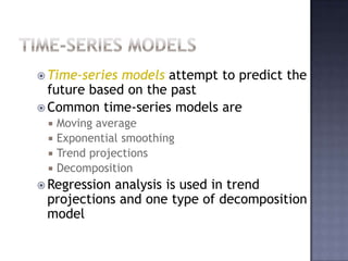
SlideShare a Scribd company logo
Lecture 6
August 16th, 2010
Forecasting
                        Techniques

Qualitative         Time-Series Methods     Causal
  Models                                   Methods


     Delphi                  Moving       Regression Analysis
     Methods                 Average

Jury of Executive          Exponential         Multiple
     Opinion                Smoothing         Regression


   Sales Force                Trend
   Composite               Projections


   Consumer
                          Decomposition
  Market Survey
 Time-series models attempt to predict the
  future based on the past
 Common time-series models are
    Moving average
    Exponential smoothing
    Trend projections
    Decomposition
 Regressionanalysis is used in trend
 projections and one type of decomposition
 model
 Causal models use variables or factors that
  might influence the quantity being
  forecasted
 The objective is to build a model with the
  best statistical relationship between the
  variable being forecast and the
  independent variables
 Regression analysis is the most common
  technique used in causal modeling
 Wacker Distributors wants to forecast sales
  for three different products
YEAR   TELEVISION SETS   RADIOS   COMPACT DISC PLAYERS
  1          250          300             110
  2          250          310             100
  3          250          320             120
  4          250          330             140
  5          250          340             170
  6          250          350             150
  7          250          360             160
  8          250          370             190
  9          250          380             200
 10          250          390             190
(a)
                                    330 –                                            Sales appear to be
                                                                                      constant over time
      Annual Sales of Televisions


                                    250 –          
                                                                                          Sales = 250
                                    200 –
                                                                                     A good estimate of
                                    150 –                                             sales in year 11 is
                                    100 –                                             250 televisions
                                     50 –
                                            |   |   |   |   |   |   |   |   |   |

                                       0 1 2 3 4 5 6 7 8 9 10
                                                    Time (Years)
(b)
                               420 –                                            Sales appear to be
                               400 –                                             increasing at a
                               380 –                                            constant rate of 10
      Annual Sales of Radios


                                                                       
                                                                   
                               360 –
                                                                                radios per year
                               340 –                       
                                                   
                                                                               Sales = 290 + 10(Year)
                               320 –           
                               300 –                                          A reasonable
                               280 –
                                                                                 estimate of sales in
                                                                                 year 11 is 400
                                       |   |   |   |   |
                                  0 1 2 3 4 5 6 7 8 9 10
                                                           |   |   |   |   |
                                                                                 televisions
                                               Time (Years)
 This trend line may
(c)                                                                                  not be perfectly
                                   200 –
                                                                                   accurate because of
      Annual Sales of CD Players


                                                                       
                                   180 –                                             variation from year
                                   160 –                                            to year
                                                                   
                                   140 –                                           Sales appear to be
                                                       
                                                                                     increasing
                                   120 –
                                                   
                                                                                   A forecast would
                                   100 –                                            probably be a larger
                                           |   |   |   |   |   |   |   |   |   |
                                                                                     figure each year
                                      0 1 2 3 4 5 6 7 8 9 10
                                                   Time (Years)
   We compare forecasted values with actual values to
    see how well one model works or to compare models

     Forecast error = Actual value – Forecast value

 One measure of accuracy is the
      mean absolute deviation (MAD)

              MAD 
                     forecast error
                           n
   Using a naïve forecasting model
            ACTUAL                     ABSOLUTE VALUE OF
          SALES OF CD   FORECAST       ERRORS (DEVIATION),
YEAR        PLAYERS       SALES       (ACTUAL – FORECAST)
 1            110          —                    —
 2            100         110            |100 – 110| = 10
 3            120         100            |120 – 110| = 20
 4            140         120            |140 – 120| = 20
 5            170         140            |170 – 140| = 30
 6            150         170            |150 – 170| = 20
 7            160         150            |160 – 150| = 10
 8            190         160            |190 – 160| = 30
 9            200         190            |200 – 190| = 10
 10           190         200            |190 – 200| = 10
 11           —           190                   —
                                       Sum of |errors| = 160
                                        MAD = 160/9 = 17.8
   Using a naïve forecasting model
               ACTUAL                   ABSOLUTE VALUE OF
             SALES OF CD   FORECAST     ERRORS (DEVIATION),
     YEAR      PLAYERS       SALES     (ACTUAL – FORECAST)
      1          110          —                  —
      2          100         110          |100 – 110| = 10
      3          120         100          |120 – 110| = 20
      4
    MAD 
      5
           forecast error  160  17.8
                 140
                 170
                             120
                             140
                                          |140 – 120| = 20
                                          |170 – 140| = 30
      6          150   n     170   9      |150 – 170| = 20
      7          160         150          |160 – 150| = 10
      8          190         160          |190 – 160| = 30
      9          200         190          |200 – 190| = 10
      10         190         200          |190 – 200| = 10
      11         —           190                 —
                                        Sum of |errors| = 160
                                         MAD = 160/9 = 17.8
 There are other popular measures of forecast
  accuracy
 The mean squared error


                MSE 
                       (error)2
                          n
 The mean absolute percent error
                      error
                     actual
             MAPE           100%
                       n
 And bias is the average error
A  time series is a sequence of evenly
  spaced events
 Time-series forecasts predict the future
  based solely of the past values of the
  variable
 Other variables are ignored
   A time series typically has four components
     1. Trend (T) is the gradual upward or downward
        movement of the data over time
     2. Seasonality (S) is a pattern of demand
        fluctuations above or below trend line that
        repeats at regular intervals
     3. Cycles (C) are patterns in annual data that
        occur every several years
     4. Random variations (R) are “blips” in the
        data caused by chance and unusual
        situations
Trend
Demand for Product or Service


                                                                           Component

                                Seasonal Peaks

                                                                                  Actual
                                                                                 Demand
                                                                                   Line
                                                                Average Demand
                                                                  over 4 Years


                                     |            |             |            |
                                    Year         Year          Year        Year
                                     1            2             3           4
                                                        Time
 There are two general forms of time-series
  models
 The multiplicative model

             Demand = T x S x C x R

 The additive model
             Demand = T + S + C + R

 Models may be combinations of these two
  forms
 Forecasters often assume errors are normally
  distributed with a mean of zero
 Moving averages can be used when demand is
  relatively steady over time
 The next forecast is the average of the most
  recent n data values from the time series
 This methods tends to smooth out short-term
  irregularities in the data series


                            Sum of demands in previous n periods
Moving average forecast 
                                            n
 Mathematically
                      Yt  Yt 1  ...  Yt  n1
            Ft 1 
                                  n

  where
          Ft 1 = forecast for time period t + 1
           Yt
             = actual value in time period t
           n = number of periods to average
 Wallace Garden Supply wants to forecast
  demand for its Storage Shed
 They have collected data for the past year
 They are using a three-month moving
  average to forecast demand (n = 3)
MONTH       ACTUAL SHED SALES   THREE-MONTH MOVING AVERAGE
January            10
February           12
March              13
April              16               (10 + 12 + 13)/3 = 11.67
May                19               (12 + 13 + 16)/3 = 13.67
June               23               (13 + 16 + 19)/3 = 16.00
July               26               (16 + 19 + 23)/3 = 19.33
August             30               (19 + 23 + 26)/3 = 22.67
September          28               (23 + 26 + 30)/3 = 26.33
October            18               (26 + 30 + 28)/3 = 28.00
November           16               (30 + 28 + 18)/3 = 25.33
December           14               (28 + 18 + 16)/3 = 20.67
January            —                (18 + 16 + 14)/3 = 16.00
 Weighted moving averages use weights to put more
  emphasis on recent periods
 Often used when a trend or other pattern is
  emerging

 Ft 1   
            ( Weight in period i )( Actual value in period)
                            ( Weights)
 Mathematically
                        w1Yt  w2Yt 1  ...  wnYt  n1
                Ft 1 
                             w1  w2  ...  wn
   where
                wi = weight for the ith observation
 Wallace Garden Supply decides to try a
       weighted moving average model to
       forecast demand for its Storage Shed
      They decide on the following weighting
       scheme
                             WEIGHTS APPLIED                   PERIOD
                                       3                 Last month
                                       2                 Two months ago
                                       1                 Three months ago
3 x Sales last month + 2 x Sales two months ago + 1 X Sales three months ago
                                       6
                                                         Sum of the weights
THREE-MONTH WEIGHTED
MONTH       ACTUAL SHED SALES          MOVING AVERAGE
January            10
February           12
March              13
April              16           [(3 X 13) + (2 X 12) + (10)]/6 = 12.17
May                19           [(3 X 16) + (2 X 13) + (12)]/6 = 14.33
June               23           [(3 X 19) + (2 X 16) + (13)]/6 = 17.00
July               26           [(3 X 23) + (2 X 19) + (16)]/6 = 20.50
August             30           [(3 X 26) + (2 X 23) + (19)]/6 = 23.83
September          28           [(3 X 30) + (2 X 26) + (23)]/6 = 27.50
October            18           [(3 X 28) + (2 X 30) + (26)]/6 = 28.33
November           16           [(3 X 18) + (2 X 28) + (30)]/6 = 23.33
December           14           [(3 X 16) + (2 X 18) + (28)]/6 = 18.67
January            —            [(3 X 14) + (2 X 16) + (18)]/6 = 15.33
 Exponential smoothing is easy to use and
      requires little record keeping of data
     It is a type of moving average

New forecast = Last period’s forecast
                   + (Last period’s actual demand - Last period’s
                   forecast)


        Where  is a weight (or smoothing
        constant) with a value between 0 and 1
        inclusive
   Mathematically

                  Ft 1  Ft   (Yt  Ft )

     where
             Ft+1 = new forecast (for time period t + 1)
              Ft = previous forecast (for time period t)
                = smoothing constant (0 ≤  ≤ 1)
               Yt = pervious period’s actual demand

 The idea is simple – the new estimate is
    the old estimate plus some fraction of
    the error in the last period
 In January, February’s demand for a certain car
  model was predicted to be 142
 Actual February demand was 153 autos
 Using a smoothing constant of  = 0.20, what is
  the forecast for March?

 New forecast (for March demand)    = 142 + 0.2(153 – 142)
                                    = 144.2 or 144 autos

 If actual demand in March was 136 autos,
    the April forecast would be
New forecast (for April demand)   = 144.2 + 0.2(136 – 144.2)
                                  = 142.6 or 143 autos
 Selecting the appropriate value for    is key
  to obtaining a good forecast
 The objective is always to generate an
  accurate forecast
 The general approach is to develop trial
  forecasts with different values of  and
  select the  that results in the lowest MAD
 Exponential smoothing forecast for two values of                     
           ACTUAL
          TONNAGE               FORECAST                     FORECAST
QUARTER   UNLOADED             USING  =0.10                USING  =0.50
   1        180      175                                       175
   2        168      175.5 = 175.00 + 0.10(180 – 175)          177.5
   3        159      174.75 = 175.50 + 0.10(168 – 175.50)      172.75
   4        175      173.18 = 174.75 + 0.10(159 – 174.75)      165.88
   5        190      173.36 = 173.18 + 0.10(175 – 173.18)      170.44
   6        205      175.02 = 173.36 + 0.10(190 – 173.36)      180.22
   7        180      178.02 = 175.02 + 0.10(205 – 175.02)      192.61
   8        182      178.22 = 178.02 + 0.10(180 – 178.02)      186.30
   9         ?       178.60 = 178.22 + 0.10(182 – 178.22)      184.15
ACTUAL                           ABSOLUTE                       ABSOLUTE
            TONNAGE       FORECAST           DEVIATIONS      FORECAST       DEVIATIONS
QUARTER     UNLOADED     WITH  = 0.10       FOR  = 0.10   WITH  = 0.50   FOR  = 0.50
    1           180             175               5…..         175               5….
    2           168             175.5             7.5..        177.5             9.5..
    3           159             174.75           15.75         172.75           13.75
    4           175             173.18            1.82         165.88            9.12
    5           190             173.36           16.64         170.44           19.56
    6           205             175.02           29.98         180.22           24.78
    7           180             178.02            1.98         192.61           12.61
    8           182             178.22            3.78         186.30            4.3..
Sum of absolute deviations                       82.45                          98.63
                             Σ|deviations|
                 MAD =                       =   10.31                  MAD =   12.33
                                  n


                       Best choice
 Like all averaging techniques, exponential
        smoothing does not respond to trends
       A more complex model can be used that adjusts
        for trends
       The basic approach is to develop an exponential
        smoothing forecast then adjust it for the trend

Forecast including trend (FITt) =   New forecast (Ft)
                                    + Trend correction (Tt)
 The equation for the trend correction uses a
  new smoothing constant 
 Tt is computed by

                Tt 1  (1  )T1   ( Ft 1  Ft )

    where
       Tt+1 = smoothed trend for period t + 1
         Tt = smoothed trend for preceding period
          =  trend smooth constant that we select
       Ft+1 = simple exponential smoothed forecast for
              period t + 1
         Ft = forecast for pervious period
 As with exponential smoothing, a high value of   
    makes the forecast more responsive to changes in
    trend
   A low value of  gives less weight to the recent
    trend and tends to smooth out the trend
   Values are generally selected using a trial-and-error
    approach based on the value of the MAD for
    different values of 
   Simple exponential smoothing is often referred to as
    first-order smoothing
   Trend-adjusted smoothing is called second-order,
    double smoothing, or Holt’s method
Trend Projection
 Trend projection fits a trend line to a series
  of historical data points
 The line is projected into the future for
  medium- to long-range forecasts
 Several trend equations can be developed
  based on exponential or quadratic models
 The simplest is a linear model developed
  using regression analysis
Trend Projection
 The mathematical form is

                 ˆ
                 Y  b0  b1 X


   where
         ˆ
        Y = predicted value
       b0 = intercept
       b1 = slope of the line
       X = time period (i.e., X = 1, 2, 3, …, n)
Trend Projection

                                                                      Dist7   *
                                                                  *
Value of Dependent Variable


                                                          Dist5           Dist6

                                              *   Dist3               *
                                                              Dist4


                              Dist1   *       Dist2
                                                          *
                                          *

                                                  Time
 Midwestern Manufacturing Company has experienced
  the following demand for it’s electrical generators
  over the period of 2001 – 2007

     YEAR          ELECTRICAL GENERATORS SOLD
      2001                       74
      2002                       79
      2003                       80
      2004                       90
      2005                      105
      2006                      142
      2007                      122
r2 says model predicts
   about 80% of the
variability in demand


Significance level for
  F-test indicates a
definite relationship
 The forecast equation is
                 ˆ
                 Y  56.71 10.54 X

 To project demand for 2008, we use the coding
  system to define X = 8
    (sales in 2008) = 56.71 + 10.54(8)
                    = 141.03, or 141 generators

 Likewise for X = 9

    (sales in 2009) = 56.71 + 10.54(9)
                    = 151.57, or 152 generators
160 –
                   150 –                                                 
                   140 –                              
                                                                        Trend Line
                   130 –                                                 ˆ
                                                                        Y  56.71 10.54 X
Generator Demand


                   120 –                                    
                   110 –
                                                 
                   100 –
                    90 –                   
                    80 –             
                    70 –                      Actual Demand Line
                    60 –
                    50 –
                            |    |    |    |     |     |    |       |     |

                           2001 2002 2003 2004 2005 2006 2007 2008 2009
                                               Year
 Recurring  variations over time may
  indicate the need for seasonal adjustments
  in the trend line
 A seasonal index indicates how a particular
  season compares with an average season
 When no trend is present, the seasonal
  index can be found by dividing the average
  value for a particular season by the
  average of all the data
 Eichler Supplies sells telephone answering
  machines
 Data has been collected for the past two
  years sales of one particular model
 They want to create a forecast this
  includes seasonality
AVERAGE
                   SALES DEMAND
                                              AVERAGE TWO-         MONTHLY     SEASONAL
MONTH            YEAR 1         YEAR 2        YEAR DEMAND          DEMAND        INDEX
January             80            100                90              94           0.957
February            85             75                80              94           0.851
March               80             90                85              94           0.904
April              110             90              100               94           1.064
May                115            131              123               94           1.309
June               120            110               115              94           1.223
July               100            110              105               94           1.117
August             110             90              100               94           1.064
September           85             95                90              94           0.957
October             75             85                80              94           0.851
November            85             75                80              94           0.851
December            80             80                80              94           0.851
                           Total average demand = 1,128
                               1,128                                Average two-year demand
Average monthly demand =               = 94     Seasonal index =
                             12 months                              Average monthly demand
   The calculations for the seasonal indices are
            1,200                         1,200
    Jan.           0.957  96    July           1.117  112
              12                            12
            1,200                         1,200
    Feb.           0.851  85    Aug.           1.064  106
              12                            12
            1,200                         1,200
    Mar.           0.904  90    Sept.          0.957  96
              12                            12
            1,200                         1,200
    Apr.           1.064  106   Oct.           0.851  85
              12                            12
            1,200                         1,200
    May            1.309  131   Nov.           0.851  85
              12                            12
            1,200                         1,200
    June           1.223  122   Dec.           0.851  85
              12                            12
Seasonal Variations with Trend
   When both trend and seasonal components are
    present, the forecasting task is more complex
   Seasonal indices should be computed using a
    centered moving average (CMA) approach
   There are four steps in computing CMAs
     1. Compute the CMA for each observation (where
        possible)
     2. Compute the seasonal ratio = Observation/CMA
        for that observation
     3. Average seasonal ratios to get seasonal indices
     4. If seasonal indices do not add to the number of
        seasons, multiply each index by (Number of
        seasons)/(Sum of indices)
Turner Industries Example
 The following are Turner Industries’ sales figures for
  the past three years

 QUARTER       YEAR 1     YEAR 2   YEAR 3     AVERAGE
     1          108       116       123         115.67
     2          125       134       142         133.67
     3          150       159       168         159.00
     4          141       152       165         152.67
  Average       131.00    140.25    149.50      140.25


                                          Seasonal
         Definite trend                    pattern
Turner Industries Example
 To calculate the CMA for quarter 3 of year 1 we
  compare the actual sales with an average quarter
  centered on that time period
 We will use 1.5 quarters before quarter 3 and 1.5
  quarters after quarter 3 – that is we take quarters 2,
  3, and 4 and one half of quarters 1, year 1 and
  quarter 1, year 2


              0.5(108) + 125 + 150 + 141 + 0.5(116)
CMA(q3, y1) =                                         = 132.00
                                4
Turner Industries Example

 We compare the actual sales in quarter 3 to
  the CMA to find the seasonal ratio

                     Sales in quarter 3 150
  Seasonal ratio                            1.136
                           CMA           132
Turner Industries Example
YEAR   QUARTER   SALES    CMA      SEASONAL RATIO
  1       1       108
          2       125
          3       150    132.000        1.136
          4       141    134.125        1.051
 2        1       116    136.375        0.851
          2       134    138.875        0.965
          3       159    141.125        1.127
          4       152    143.000        1.063
 3        1       123    145.125        0.848
          2       142    147.875        0.960
          3       168
          4       165
Turner Industries Example
 There are two seasonal ratios for each quarter so
  these are averaged to get the seasonal index

   Index for   quarter   1   =   I1   =   (0.851   +   0.848)/2   =   0.85
   Index for   quarter   2   =   I2   =   (0.965   +   0.960)/2   =   0.96
   Index for   quarter   3   =   I3   =   (1.136   +   1.127)/2   =   1.13
   Index for   quarter   4   =   I4   =   (1.051   +   1.063)/2   =   1.06
Turner Industries Example

 Scatter plot of Turner Industries data and
        CMAs
        200 –                             CMA

        150 –                                                                       
                                                                          
                                                                  
        100 –                            
Sales


         50 –
                              Original Sales Figures
          0–      |       |     |     |       |       |    |    |       |       |     |    |

                  1       2     3     4     5   6    7          8       9       10    11   12
                                           Time Period
   Decomposition is the process of isolating linear
    trend and seasonal factors to develop more accurate
    forecasts
   There are five steps to decomposition
     1. Compute seasonal indices using CMAs
     2. Deseasonalize the data by dividing each number
        by its seasonal index
     3. Find the equation of a trend line using the
        deseasonalized data
     4. Forecast for future periods using the trend line
     5. Multiply the trend line forecast by the
        appropriate seasonal index
SALES        SEASONAL   DESEASONALIZED
($1,000,000s)     INDEX    SALES ($1,000,000s)
     108           0.85         127.059
     125           0.96         130.208
     150           1.13         132.743
     141           1.06         133.019
     116           0.85         136.471
     134           0.96         139.583
     159           1.13         140.708
     152           1.06         143.396
     123           0.85         144.706
     142           0.96         147.917
     168           1.13         148.673
     165           1.06         155.660
 Find a trend line using the deseasonalized data

               b1 = 2.34     b0 = 124.78
 Develop a forecast using this trend a multiply the
  forecast by the appropriate seasonal index
      ˆ
     Y = 124.78 + 2.34X
        = 124.78 + 2.34(13)
        = 155.2 (forecast before adjustment for
                seasonality)
      ˆ
     Y x I1 = 155.2 x 0.85 = 131.92
 A San Diego hospital used 66 months of adult
   inpatient days to develop the following seasonal
   indices

  MONTH    SEASONALITY INDEX     MONTH     SEASONALITY INDEX
January          1.0436        July              1.0302
February         0.9669        August            1.0405
March            1.0203        September         0.9653
April            1.0087        October           1.0048
May              0.9935        November          0.9598
June             0.9906        December          0.9805
 Using this data they developed the following
  equation
                   ˆ
                  Y = 8,091 + 21.5X
  where
               ˆ
              Y = forecast patient days
              X = time in months

 Based on this model, the forecast for patient days
  for the next period (67) is

Patient days = 8,091 + (21.5)(67) = 9,532 (trend only)
Patient days = (9,532)(1.0436)
             = 9,948 (trend and seasonal)
   Multiple regression can be used to forecast both
    trend and seasonal components in a time series
       One independent variable is time
       Dummy independent variables are used to represent the
        seasons
   The model is an additive decomposition model
                 ˆ
                 Y  a  b1 X 1  b2 X 2  b3 X 3  b4 X 4
        where
                    X1   = time period
                    X2   = 1 if quarter 2, 0 otherwise
                    X3   = 1 if quarter 3, 0 otherwise
                    X4   = 1 if quarter 4, 0 otherwise
   The resulting regression equation is

        ˆ
        Y  104.1  2.3 X 1  15.7 X 2  38.7 X 3  30.1X 4

 Using the model to forecast sales for the first two
    quarters of next year
    ˆ
    Y  104.1  2.3(13)  15.7(0)  38.7(0)  30.1(0)  134
     ˆ
    Y  104.1  2.3(14 )  15.7(1)  38.7(0)  30.1(0)  152

 These are different from the results obtained using
  the multiplicative decomposition method
 Use MAD and MSE to determine the best model
 Tracking signals can be used to monitor the
      performance of a forecast
     Tacking signals are computed using the following
      equation

                                        RSFE
                      Tracking signal 
                                        MAD

       where

                     MAD 
                            forecast error
                                       n
RSFE = Ratio of running sum of forecast errors
     = ∑(actual demand in period i - forecast demand in period i)
Signal Tripped
         Upper Control Limit                    Tracking Signal
   +

                                                Acceptable
0 MADs                                          Range

   –
         Lower Control Limit


                        Time
 Positive tracking signals indicate demand is greater
    than forecast
   Negative tracking signals indicate demand is less
    than forecast
   Some variation is expected, but a good forecast will
    have about as much positive error as negative error
   Problems are indicated when the signal trips either
    the upper or lower predetermined limits
   This indicates there has been an unacceptable
    amount of variation
   Limits should be reasonable and may vary from item
    to item
 Tracking signal for quarterly sales of croissants


 TIME    FORECAST   ACTUAL                  |FORECAST |   CUMULATIVE          TRACKING
PERIOD    DEMAND    DEMAND   ERROR   RSFE   | ERROR |       ERROR      MAD     SIGNAL
  1        100        90      –10     –10      10             10       10.0      –1
  2        100        95       –5     –15       5             15        7.5      –2
  3        100        115     +15       0      15             30       10.0       0
  4        110        100     –10     –10      10             40       10.0      –1
  5        110        125     +15      +5      15             55       11.0     +0.5
  6        110        140     +30     +35      35             85       14.2     +2.5


                 MAD 
                        forecast error  85  14.2
                             n        6
                             RSFE 35
           Tracking signal           2.5MAD s
                             MAD 14.2
 Adaptive smoothing is the computer monitoring
  of tracking signals and self-adjustment if a limit
  is tripped
 In exponential smoothing, the values of  and 
  are adjusted when the computer detects an
  excessive amount of variation
 Spreadsheets can be used by small and medium-
  sized forecasting problems
 More advanced programs (SAS, SPSS, Minitab)
  handle time-series and causal models
 May automatically select best model parameters
 Dedicated forecasting packages may be fully
  automatic
 May be integrated with inventory planning and
  control
 39 students
 Average:
    3.43
 High:
    14.50 100% class grade
 Grade
    A >= 85%
    B >= 70%, < 85%
    C >= 60%, < 70%
    D >= 50%, < 60%
    F < 50%

More Related Content

What's hot

Chapter 1 introduction
Chapter 1   introductionChapter 1   introduction
Terms of trades
Terms of tradesTerms of trades
Terms of trades
Vinod Yadav
 
Shifts In Demand And Supply And Market Equilibrium
Shifts In Demand And Supply And Market EquilibriumShifts In Demand And Supply And Market Equilibrium
Shifts In Demand And Supply And Market Equilibrium
Shikhar Bafna
 
Premise control
Premise control Premise control
Premise control
Anand Verma
 
Lecture 7 - Endogenous growth theory
Lecture 7 - Endogenous growth theoryLecture 7 - Endogenous growth theory
Lecture 7 - Endogenous growth theoryUNU.MERIT
 
Cost of capital
Cost of capitalCost of capital
Cost of capital
mahadeva prasad
 
Ratio Analysis
Ratio AnalysisRatio Analysis
Ratio Analysis
engineer sood
 
Capital Budgeting
Capital BudgetingCapital Budgeting
Capital Budgeting
sabbir mahmood
 
Modigliani & Miller Approach
Modigliani & Miller ApproachModigliani & Miller Approach
Modigliani & Miller Approach
Sunanda Priyadarshini
 
Cash and Receivable Management.pptx
Cash and Receivable Management.pptxCash and Receivable Management.pptx
Cash and Receivable Management.pptx
AbhayKhane1
 
Evaluation of merger
Evaluation of mergerEvaluation of merger
Evaluation of merger
shireesha pallepati
 
Technical analysis OF STOCK MARKET presentation of mba 4 sem FINANCE PPT
Technical analysis OF STOCK MARKET  presentation of mba 4 sem FINANCE PPTTechnical analysis OF STOCK MARKET  presentation of mba 4 sem FINANCE PPT
Technical analysis OF STOCK MARKET presentation of mba 4 sem FINANCE PPT
Babasab Patil
 
Hallmarks of research
Hallmarks of researchHallmarks of research
Hallmarks of research
Subhanullah Khan BBA,MBA,
 

What's hot (14)

Chapter 1 introduction
Chapter 1   introductionChapter 1   introduction
Chapter 1 introduction
 
Terms of trades
Terms of tradesTerms of trades
Terms of trades
 
Shifts In Demand And Supply And Market Equilibrium
Shifts In Demand And Supply And Market EquilibriumShifts In Demand And Supply And Market Equilibrium
Shifts In Demand And Supply And Market Equilibrium
 
Premise control
Premise control Premise control
Premise control
 
Lecture 7 - Endogenous growth theory
Lecture 7 - Endogenous growth theoryLecture 7 - Endogenous growth theory
Lecture 7 - Endogenous growth theory
 
Cost of capital
Cost of capitalCost of capital
Cost of capital
 
Ratio Analysis
Ratio AnalysisRatio Analysis
Ratio Analysis
 
Capital Budgeting
Capital BudgetingCapital Budgeting
Capital Budgeting
 
Modigliani & Miller Approach
Modigliani & Miller ApproachModigliani & Miller Approach
Modigliani & Miller Approach
 
Lecture 3
Lecture 3Lecture 3
Lecture 3
 
Cash and Receivable Management.pptx
Cash and Receivable Management.pptxCash and Receivable Management.pptx
Cash and Receivable Management.pptx
 
Evaluation of merger
Evaluation of mergerEvaluation of merger
Evaluation of merger
 
Technical analysis OF STOCK MARKET presentation of mba 4 sem FINANCE PPT
Technical analysis OF STOCK MARKET  presentation of mba 4 sem FINANCE PPTTechnical analysis OF STOCK MARKET  presentation of mba 4 sem FINANCE PPT
Technical analysis OF STOCK MARKET presentation of mba 4 sem FINANCE PPT
 
Hallmarks of research
Hallmarks of researchHallmarks of research
Hallmarks of research
 

Viewers also liked

IBM401 Lecture 9
IBM401 Lecture 9IBM401 Lecture 9
IBM401 Lecture 9saark
 
IBM401 Lecture 8
IBM401 Lecture 8IBM401 Lecture 8
IBM401 Lecture 8saark
 
IBM401 Lecture 7
IBM401 Lecture 7IBM401 Lecture 7
IBM401 Lecture 7saark
 
IBE303 Lecture 7
IBE303 Lecture 7IBE303 Lecture 7
IBE303 Lecture 7saark
 
IBE303 Lecture 12
IBE303 Lecture 12IBE303 Lecture 12
IBE303 Lecture 12saark
 
IBE303 Midterm key
IBE303 Midterm keyIBE303 Midterm key
IBE303 Midterm keysaark
 
IBM401 Midterm key
IBM401 Midterm keyIBM401 Midterm key
IBM401 Midterm keysaark
 
Ibe303 grade
Ibe303 gradeIbe303 grade
Ibe303 gradesaark
 
IBM401 Lecture 5
IBM401 Lecture 5IBM401 Lecture 5
IBM401 Lecture 5saark
 
IBE303 Lecture 10
IBE303 Lecture 10IBE303 Lecture 10
IBE303 Lecture 10saark
 
IBM401 Lecture 10
IBM401 Lecture 10IBM401 Lecture 10
IBM401 Lecture 10saark
 
IBE303 International Economic Lecture 4
IBE303 International Economic Lecture 4IBE303 International Economic Lecture 4
IBE303 International Economic Lecture 4saark
 
IBE303 - Lecture 6
IBE303 - Lecture 6IBE303 - Lecture 6
IBE303 - Lecture 6saark
 
IBE303 Lecture 5
IBE303 Lecture 5IBE303 Lecture 5
IBE303 Lecture 5saark
 

Viewers also liked (14)

IBM401 Lecture 9
IBM401 Lecture 9IBM401 Lecture 9
IBM401 Lecture 9
 
IBM401 Lecture 8
IBM401 Lecture 8IBM401 Lecture 8
IBM401 Lecture 8
 
IBM401 Lecture 7
IBM401 Lecture 7IBM401 Lecture 7
IBM401 Lecture 7
 
IBE303 Lecture 7
IBE303 Lecture 7IBE303 Lecture 7
IBE303 Lecture 7
 
IBE303 Lecture 12
IBE303 Lecture 12IBE303 Lecture 12
IBE303 Lecture 12
 
IBE303 Midterm key
IBE303 Midterm keyIBE303 Midterm key
IBE303 Midterm key
 
IBM401 Midterm key
IBM401 Midterm keyIBM401 Midterm key
IBM401 Midterm key
 
Ibe303 grade
Ibe303 gradeIbe303 grade
Ibe303 grade
 
IBM401 Lecture 5
IBM401 Lecture 5IBM401 Lecture 5
IBM401 Lecture 5
 
IBE303 Lecture 10
IBE303 Lecture 10IBE303 Lecture 10
IBE303 Lecture 10
 
IBM401 Lecture 10
IBM401 Lecture 10IBM401 Lecture 10
IBM401 Lecture 10
 
IBE303 International Economic Lecture 4
IBE303 International Economic Lecture 4IBE303 International Economic Lecture 4
IBE303 International Economic Lecture 4
 
IBE303 - Lecture 6
IBE303 - Lecture 6IBE303 - Lecture 6
IBE303 - Lecture 6
 
IBE303 Lecture 5
IBE303 Lecture 5IBE303 Lecture 5
IBE303 Lecture 5
 

More from saark

Ibm401 grade
Ibm401 gradeIbm401 grade
Ibm401 gradesaark
 
IBM401 Lecture 12
IBM401 Lecture 12IBM401 Lecture 12
IBM401 Lecture 12saark
 
IBM401 Lecture 11
IBM401 Lecture 11IBM401 Lecture 11
IBM401 Lecture 11saark
 
IBE303 Lecture 11
IBE303 Lecture 11IBE303 Lecture 11
IBE303 Lecture 11saark
 
IBE303 Lecture 9
IBE303 Lecture 9IBE303 Lecture 9
IBE303 Lecture 9saark
 
IBE303 Lecture 8
IBE303 Lecture 8IBE303 Lecture 8
IBE303 Lecture 8saark
 
IBM401 Assignment
IBM401 AssignmentIBM401 Assignment
IBM401 Assignmentsaark
 
Business Quantitative Lecture 3
Business Quantitative Lecture 3Business Quantitative Lecture 3
Business Quantitative Lecture 3saark
 
IBE303 Assignment
IBE303 AssignmentIBE303 Assignment
IBE303 Assignmentsaark
 
International Economic Lecture 3
International Economic Lecture 3International Economic Lecture 3
International Economic Lecture 3
saark
 
International Economic Lecture 2
International Economic Lecture 2International Economic Lecture 2
International Economic Lecture 2
saark
 
Business Quantitative - Lecture 2
Business Quantitative - Lecture 2Business Quantitative - Lecture 2
Business Quantitative - Lecture 2
saark
 

More from saark (12)

Ibm401 grade
Ibm401 gradeIbm401 grade
Ibm401 grade
 
IBM401 Lecture 12
IBM401 Lecture 12IBM401 Lecture 12
IBM401 Lecture 12
 
IBM401 Lecture 11
IBM401 Lecture 11IBM401 Lecture 11
IBM401 Lecture 11
 
IBE303 Lecture 11
IBE303 Lecture 11IBE303 Lecture 11
IBE303 Lecture 11
 
IBE303 Lecture 9
IBE303 Lecture 9IBE303 Lecture 9
IBE303 Lecture 9
 
IBE303 Lecture 8
IBE303 Lecture 8IBE303 Lecture 8
IBE303 Lecture 8
 
IBM401 Assignment
IBM401 AssignmentIBM401 Assignment
IBM401 Assignment
 
Business Quantitative Lecture 3
Business Quantitative Lecture 3Business Quantitative Lecture 3
Business Quantitative Lecture 3
 
IBE303 Assignment
IBE303 AssignmentIBE303 Assignment
IBE303 Assignment
 
International Economic Lecture 3
International Economic Lecture 3International Economic Lecture 3
International Economic Lecture 3
 
International Economic Lecture 2
International Economic Lecture 2International Economic Lecture 2
International Economic Lecture 2
 
Business Quantitative - Lecture 2
Business Quantitative - Lecture 2Business Quantitative - Lecture 2
Business Quantitative - Lecture 2
 

IBM401 - Lecture 6

  • 2. Forecasting Techniques Qualitative Time-Series Methods Causal Models Methods Delphi Moving Regression Analysis Methods Average Jury of Executive Exponential Multiple Opinion Smoothing Regression Sales Force Trend Composite Projections Consumer Decomposition Market Survey
  • 3.  Time-series models attempt to predict the future based on the past  Common time-series models are  Moving average  Exponential smoothing  Trend projections  Decomposition  Regressionanalysis is used in trend projections and one type of decomposition model
  • 4.  Causal models use variables or factors that might influence the quantity being forecasted  The objective is to build a model with the best statistical relationship between the variable being forecast and the independent variables  Regression analysis is the most common technique used in causal modeling
  • 5.  Wacker Distributors wants to forecast sales for three different products YEAR TELEVISION SETS RADIOS COMPACT DISC PLAYERS 1 250 300 110 2 250 310 100 3 250 320 120 4 250 330 140 5 250 340 170 6 250 350 150 7 250 360 160 8 250 370 190 9 250 380 200 10 250 390 190
  • 6. (a) 330 –  Sales appear to be constant over time Annual Sales of Televisions 250 –           Sales = 250 200 –  A good estimate of 150 – sales in year 11 is 100 – 250 televisions 50 – | | | | | | | | | | 0 1 2 3 4 5 6 7 8 9 10 Time (Years)
  • 7. (b) 420 –  Sales appear to be 400 – increasing at a 380 –  constant rate of 10 Annual Sales of Radios   360 –  radios per year 340 –    Sales = 290 + 10(Year) 320 –  300 –    A reasonable 280 – estimate of sales in year 11 is 400 | | | | | 0 1 2 3 4 5 6 7 8 9 10 | | | | | televisions Time (Years)
  • 8.  This trend line may (c) not be perfectly 200 –   accurate because of Annual Sales of CD Players  180 – variation from year 160 –  to year  140 –   Sales appear to be  increasing 120 –    A forecast would 100 –  probably be a larger | | | | | | | | | | figure each year 0 1 2 3 4 5 6 7 8 9 10 Time (Years)
  • 9. We compare forecasted values with actual values to see how well one model works or to compare models Forecast error = Actual value – Forecast value  One measure of accuracy is the  mean absolute deviation (MAD) MAD   forecast error n
  • 10. Using a naïve forecasting model ACTUAL ABSOLUTE VALUE OF SALES OF CD FORECAST ERRORS (DEVIATION), YEAR PLAYERS SALES (ACTUAL – FORECAST) 1 110 — — 2 100 110 |100 – 110| = 10 3 120 100 |120 – 110| = 20 4 140 120 |140 – 120| = 20 5 170 140 |170 – 140| = 30 6 150 170 |150 – 170| = 20 7 160 150 |160 – 150| = 10 8 190 160 |190 – 160| = 30 9 200 190 |200 – 190| = 10 10 190 200 |190 – 200| = 10 11 — 190 — Sum of |errors| = 160 MAD = 160/9 = 17.8
  • 11. Using a naïve forecasting model ACTUAL ABSOLUTE VALUE OF SALES OF CD FORECAST ERRORS (DEVIATION), YEAR PLAYERS SALES (ACTUAL – FORECAST) 1 110 — — 2 100 110 |100 – 110| = 10 3 120 100 |120 – 110| = 20 4 MAD  5  forecast error  160  17.8 140 170 120 140 |140 – 120| = 20 |170 – 140| = 30 6 150 n 170 9 |150 – 170| = 20 7 160 150 |160 – 150| = 10 8 190 160 |190 – 160| = 30 9 200 190 |200 – 190| = 10 10 190 200 |190 – 200| = 10 11 — 190 — Sum of |errors| = 160 MAD = 160/9 = 17.8
  • 12.  There are other popular measures of forecast accuracy  The mean squared error MSE   (error)2 n  The mean absolute percent error error  actual MAPE  100% n  And bias is the average error
  • 13. A time series is a sequence of evenly spaced events  Time-series forecasts predict the future based solely of the past values of the variable  Other variables are ignored
  • 14. A time series typically has four components 1. Trend (T) is the gradual upward or downward movement of the data over time 2. Seasonality (S) is a pattern of demand fluctuations above or below trend line that repeats at regular intervals 3. Cycles (C) are patterns in annual data that occur every several years 4. Random variations (R) are “blips” in the data caused by chance and unusual situations
  • 15. Trend Demand for Product or Service Component Seasonal Peaks Actual Demand Line Average Demand over 4 Years | | | | Year Year Year Year 1 2 3 4 Time
  • 16.  There are two general forms of time-series models  The multiplicative model Demand = T x S x C x R  The additive model Demand = T + S + C + R  Models may be combinations of these two forms  Forecasters often assume errors are normally distributed with a mean of zero
  • 17.  Moving averages can be used when demand is relatively steady over time  The next forecast is the average of the most recent n data values from the time series  This methods tends to smooth out short-term irregularities in the data series Sum of demands in previous n periods Moving average forecast  n
  • 18.  Mathematically Yt  Yt 1  ...  Yt  n1 Ft 1  n where Ft 1 = forecast for time period t + 1 Yt = actual value in time period t n = number of periods to average
  • 19.
  • 20.  Wallace Garden Supply wants to forecast demand for its Storage Shed  They have collected data for the past year  They are using a three-month moving average to forecast demand (n = 3)
  • 21. MONTH ACTUAL SHED SALES THREE-MONTH MOVING AVERAGE January 10 February 12 March 13 April 16 (10 + 12 + 13)/3 = 11.67 May 19 (12 + 13 + 16)/3 = 13.67 June 23 (13 + 16 + 19)/3 = 16.00 July 26 (16 + 19 + 23)/3 = 19.33 August 30 (19 + 23 + 26)/3 = 22.67 September 28 (23 + 26 + 30)/3 = 26.33 October 18 (26 + 30 + 28)/3 = 28.00 November 16 (30 + 28 + 18)/3 = 25.33 December 14 (28 + 18 + 16)/3 = 20.67 January — (18 + 16 + 14)/3 = 16.00
  • 22.  Weighted moving averages use weights to put more emphasis on recent periods  Often used when a trend or other pattern is emerging Ft 1   ( Weight in period i )( Actual value in period)  ( Weights)  Mathematically w1Yt  w2Yt 1  ...  wnYt  n1 Ft 1  w1  w2  ...  wn where wi = weight for the ith observation
  • 23.
  • 24.  Wallace Garden Supply decides to try a weighted moving average model to forecast demand for its Storage Shed  They decide on the following weighting scheme WEIGHTS APPLIED PERIOD 3 Last month 2 Two months ago 1 Three months ago 3 x Sales last month + 2 x Sales two months ago + 1 X Sales three months ago 6 Sum of the weights
  • 25. THREE-MONTH WEIGHTED MONTH ACTUAL SHED SALES MOVING AVERAGE January 10 February 12 March 13 April 16 [(3 X 13) + (2 X 12) + (10)]/6 = 12.17 May 19 [(3 X 16) + (2 X 13) + (12)]/6 = 14.33 June 23 [(3 X 19) + (2 X 16) + (13)]/6 = 17.00 July 26 [(3 X 23) + (2 X 19) + (16)]/6 = 20.50 August 30 [(3 X 26) + (2 X 23) + (19)]/6 = 23.83 September 28 [(3 X 30) + (2 X 26) + (23)]/6 = 27.50 October 18 [(3 X 28) + (2 X 30) + (26)]/6 = 28.33 November 16 [(3 X 18) + (2 X 28) + (30)]/6 = 23.33 December 14 [(3 X 16) + (2 X 18) + (28)]/6 = 18.67 January — [(3 X 14) + (2 X 16) + (18)]/6 = 15.33
  • 26.
  • 27.
  • 28.  Exponential smoothing is easy to use and requires little record keeping of data  It is a type of moving average New forecast = Last period’s forecast + (Last period’s actual demand - Last period’s forecast) Where  is a weight (or smoothing constant) with a value between 0 and 1 inclusive
  • 29. Mathematically Ft 1  Ft   (Yt  Ft ) where Ft+1 = new forecast (for time period t + 1) Ft = previous forecast (for time period t)  = smoothing constant (0 ≤  ≤ 1) Yt = pervious period’s actual demand  The idea is simple – the new estimate is the old estimate plus some fraction of the error in the last period
  • 30.
  • 31.  In January, February’s demand for a certain car model was predicted to be 142  Actual February demand was 153 autos  Using a smoothing constant of  = 0.20, what is the forecast for March? New forecast (for March demand) = 142 + 0.2(153 – 142) = 144.2 or 144 autos  If actual demand in March was 136 autos, the April forecast would be New forecast (for April demand) = 144.2 + 0.2(136 – 144.2) = 142.6 or 143 autos
  • 32.  Selecting the appropriate value for  is key to obtaining a good forecast  The objective is always to generate an accurate forecast  The general approach is to develop trial forecasts with different values of  and select the  that results in the lowest MAD
  • 33.
  • 34.  Exponential smoothing forecast for two values of  ACTUAL TONNAGE FORECAST FORECAST QUARTER UNLOADED USING  =0.10 USING  =0.50 1 180 175 175 2 168 175.5 = 175.00 + 0.10(180 – 175) 177.5 3 159 174.75 = 175.50 + 0.10(168 – 175.50) 172.75 4 175 173.18 = 174.75 + 0.10(159 – 174.75) 165.88 5 190 173.36 = 173.18 + 0.10(175 – 173.18) 170.44 6 205 175.02 = 173.36 + 0.10(190 – 173.36) 180.22 7 180 178.02 = 175.02 + 0.10(205 – 175.02) 192.61 8 182 178.22 = 178.02 + 0.10(180 – 178.02) 186.30 9 ? 178.60 = 178.22 + 0.10(182 – 178.22) 184.15
  • 35. ACTUAL ABSOLUTE ABSOLUTE TONNAGE FORECAST DEVIATIONS FORECAST DEVIATIONS QUARTER UNLOADED WITH  = 0.10 FOR  = 0.10 WITH  = 0.50 FOR  = 0.50 1 180 175 5….. 175 5…. 2 168 175.5 7.5.. 177.5 9.5.. 3 159 174.75 15.75 172.75 13.75 4 175 173.18 1.82 165.88 9.12 5 190 173.36 16.64 170.44 19.56 6 205 175.02 29.98 180.22 24.78 7 180 178.02 1.98 192.61 12.61 8 182 178.22 3.78 186.30 4.3.. Sum of absolute deviations 82.45 98.63 Σ|deviations| MAD = = 10.31 MAD = 12.33 n Best choice
  • 36.
  • 37.
  • 38.  Like all averaging techniques, exponential smoothing does not respond to trends  A more complex model can be used that adjusts for trends  The basic approach is to develop an exponential smoothing forecast then adjust it for the trend Forecast including trend (FITt) = New forecast (Ft) + Trend correction (Tt)
  • 39.  The equation for the trend correction uses a new smoothing constant   Tt is computed by Tt 1  (1  )T1   ( Ft 1  Ft ) where Tt+1 = smoothed trend for period t + 1 Tt = smoothed trend for preceding period = trend smooth constant that we select Ft+1 = simple exponential smoothed forecast for period t + 1 Ft = forecast for pervious period
  • 40.  As with exponential smoothing, a high value of  makes the forecast more responsive to changes in trend  A low value of  gives less weight to the recent trend and tends to smooth out the trend  Values are generally selected using a trial-and-error approach based on the value of the MAD for different values of   Simple exponential smoothing is often referred to as first-order smoothing  Trend-adjusted smoothing is called second-order, double smoothing, or Holt’s method
  • 41. Trend Projection  Trend projection fits a trend line to a series of historical data points  The line is projected into the future for medium- to long-range forecasts  Several trend equations can be developed based on exponential or quadratic models  The simplest is a linear model developed using regression analysis
  • 42. Trend Projection  The mathematical form is ˆ Y  b0  b1 X where ˆ Y = predicted value b0 = intercept b1 = slope of the line X = time period (i.e., X = 1, 2, 3, …, n)
  • 43. Trend Projection Dist7 * * Value of Dependent Variable Dist5 Dist6 * Dist3 * Dist4 Dist1 * Dist2 * * Time
  • 44.
  • 45.  Midwestern Manufacturing Company has experienced the following demand for it’s electrical generators over the period of 2001 – 2007 YEAR ELECTRICAL GENERATORS SOLD 2001 74 2002 79 2003 80 2004 90 2005 105 2006 142 2007 122
  • 46. r2 says model predicts about 80% of the variability in demand Significance level for F-test indicates a definite relationship
  • 47.  The forecast equation is ˆ Y  56.71 10.54 X  To project demand for 2008, we use the coding system to define X = 8 (sales in 2008) = 56.71 + 10.54(8) = 141.03, or 141 generators  Likewise for X = 9 (sales in 2009) = 56.71 + 10.54(9) = 151.57, or 152 generators
  • 48. 160 – 150 –  140 –  Trend Line 130 – ˆ Y  56.71 10.54 X Generator Demand 120 –  110 –  100 – 90 –  80 –   70 –  Actual Demand Line 60 – 50 – | | | | | | | | | 2001 2002 2003 2004 2005 2006 2007 2008 2009 Year
  • 49.  Recurring variations over time may indicate the need for seasonal adjustments in the trend line  A seasonal index indicates how a particular season compares with an average season  When no trend is present, the seasonal index can be found by dividing the average value for a particular season by the average of all the data
  • 50.
  • 51.  Eichler Supplies sells telephone answering machines  Data has been collected for the past two years sales of one particular model  They want to create a forecast this includes seasonality
  • 52. AVERAGE SALES DEMAND AVERAGE TWO- MONTHLY SEASONAL MONTH YEAR 1 YEAR 2 YEAR DEMAND DEMAND INDEX January 80 100 90 94 0.957 February 85 75 80 94 0.851 March 80 90 85 94 0.904 April 110 90 100 94 1.064 May 115 131 123 94 1.309 June 120 110 115 94 1.223 July 100 110 105 94 1.117 August 110 90 100 94 1.064 September 85 95 90 94 0.957 October 75 85 80 94 0.851 November 85 75 80 94 0.851 December 80 80 80 94 0.851 Total average demand = 1,128 1,128 Average two-year demand Average monthly demand = = 94 Seasonal index = 12 months Average monthly demand
  • 53. The calculations for the seasonal indices are 1,200 1,200 Jan.  0.957  96 July  1.117  112 12 12 1,200 1,200 Feb.  0.851  85 Aug.  1.064  106 12 12 1,200 1,200 Mar.  0.904  90 Sept.  0.957  96 12 12 1,200 1,200 Apr.  1.064  106 Oct.  0.851  85 12 12 1,200 1,200 May  1.309  131 Nov.  0.851  85 12 12 1,200 1,200 June  1.223  122 Dec.  0.851  85 12 12
  • 54. Seasonal Variations with Trend  When both trend and seasonal components are present, the forecasting task is more complex  Seasonal indices should be computed using a centered moving average (CMA) approach  There are four steps in computing CMAs 1. Compute the CMA for each observation (where possible) 2. Compute the seasonal ratio = Observation/CMA for that observation 3. Average seasonal ratios to get seasonal indices 4. If seasonal indices do not add to the number of seasons, multiply each index by (Number of seasons)/(Sum of indices)
  • 55.
  • 56. Turner Industries Example  The following are Turner Industries’ sales figures for the past three years QUARTER YEAR 1 YEAR 2 YEAR 3 AVERAGE 1 108 116 123 115.67 2 125 134 142 133.67 3 150 159 168 159.00 4 141 152 165 152.67 Average 131.00 140.25 149.50 140.25 Seasonal Definite trend pattern
  • 57. Turner Industries Example  To calculate the CMA for quarter 3 of year 1 we compare the actual sales with an average quarter centered on that time period  We will use 1.5 quarters before quarter 3 and 1.5 quarters after quarter 3 – that is we take quarters 2, 3, and 4 and one half of quarters 1, year 1 and quarter 1, year 2 0.5(108) + 125 + 150 + 141 + 0.5(116) CMA(q3, y1) = = 132.00 4
  • 58. Turner Industries Example  We compare the actual sales in quarter 3 to the CMA to find the seasonal ratio Sales in quarter 3 150 Seasonal ratio    1.136 CMA 132
  • 59. Turner Industries Example YEAR QUARTER SALES CMA SEASONAL RATIO 1 1 108 2 125 3 150 132.000 1.136 4 141 134.125 1.051 2 1 116 136.375 0.851 2 134 138.875 0.965 3 159 141.125 1.127 4 152 143.000 1.063 3 1 123 145.125 0.848 2 142 147.875 0.960 3 168 4 165
  • 60. Turner Industries Example  There are two seasonal ratios for each quarter so these are averaged to get the seasonal index Index for quarter 1 = I1 = (0.851 + 0.848)/2 = 0.85 Index for quarter 2 = I2 = (0.965 + 0.960)/2 = 0.96 Index for quarter 3 = I3 = (1.136 + 1.127)/2 = 1.13 Index for quarter 4 = I4 = (1.051 + 1.063)/2 = 1.06
  • 61. Turner Industries Example  Scatter plot of Turner Industries data and CMAs 200 – CMA 150 –           100 –   Sales 50 – Original Sales Figures 0– | | | | | | | | | | | | 1 2 3 4 5 6 7 8 9 10 11 12 Time Period
  • 62. Decomposition is the process of isolating linear trend and seasonal factors to develop more accurate forecasts  There are five steps to decomposition 1. Compute seasonal indices using CMAs 2. Deseasonalize the data by dividing each number by its seasonal index 3. Find the equation of a trend line using the deseasonalized data 4. Forecast for future periods using the trend line 5. Multiply the trend line forecast by the appropriate seasonal index
  • 63.
  • 64. SALES SEASONAL DESEASONALIZED ($1,000,000s) INDEX SALES ($1,000,000s) 108 0.85 127.059 125 0.96 130.208 150 1.13 132.743 141 1.06 133.019 116 0.85 136.471 134 0.96 139.583 159 1.13 140.708 152 1.06 143.396 123 0.85 144.706 142 0.96 147.917 168 1.13 148.673 165 1.06 155.660
  • 65.  Find a trend line using the deseasonalized data b1 = 2.34 b0 = 124.78  Develop a forecast using this trend a multiply the forecast by the appropriate seasonal index ˆ Y = 124.78 + 2.34X = 124.78 + 2.34(13) = 155.2 (forecast before adjustment for seasonality) ˆ Y x I1 = 155.2 x 0.85 = 131.92
  • 66.
  • 67.  A San Diego hospital used 66 months of adult inpatient days to develop the following seasonal indices MONTH SEASONALITY INDEX MONTH SEASONALITY INDEX January 1.0436 July 1.0302 February 0.9669 August 1.0405 March 1.0203 September 0.9653 April 1.0087 October 1.0048 May 0.9935 November 0.9598 June 0.9906 December 0.9805
  • 68.  Using this data they developed the following equation ˆ Y = 8,091 + 21.5X where ˆ Y = forecast patient days X = time in months  Based on this model, the forecast for patient days for the next period (67) is Patient days = 8,091 + (21.5)(67) = 9,532 (trend only) Patient days = (9,532)(1.0436) = 9,948 (trend and seasonal)
  • 69. Multiple regression can be used to forecast both trend and seasonal components in a time series  One independent variable is time  Dummy independent variables are used to represent the seasons  The model is an additive decomposition model ˆ Y  a  b1 X 1  b2 X 2  b3 X 3  b4 X 4 where X1 = time period X2 = 1 if quarter 2, 0 otherwise X3 = 1 if quarter 3, 0 otherwise X4 = 1 if quarter 4, 0 otherwise
  • 70.
  • 71.
  • 72. The resulting regression equation is ˆ Y  104.1  2.3 X 1  15.7 X 2  38.7 X 3  30.1X 4  Using the model to forecast sales for the first two quarters of next year ˆ Y  104.1  2.3(13)  15.7(0)  38.7(0)  30.1(0)  134 ˆ Y  104.1  2.3(14 )  15.7(1)  38.7(0)  30.1(0)  152  These are different from the results obtained using the multiplicative decomposition method  Use MAD and MSE to determine the best model
  • 73.  Tracking signals can be used to monitor the performance of a forecast  Tacking signals are computed using the following equation RSFE Tracking signal  MAD where MAD   forecast error n RSFE = Ratio of running sum of forecast errors = ∑(actual demand in period i - forecast demand in period i)
  • 74. Signal Tripped Upper Control Limit Tracking Signal + Acceptable 0 MADs Range – Lower Control Limit Time
  • 75.  Positive tracking signals indicate demand is greater than forecast  Negative tracking signals indicate demand is less than forecast  Some variation is expected, but a good forecast will have about as much positive error as negative error  Problems are indicated when the signal trips either the upper or lower predetermined limits  This indicates there has been an unacceptable amount of variation  Limits should be reasonable and may vary from item to item
  • 76.
  • 77.  Tracking signal for quarterly sales of croissants TIME FORECAST ACTUAL |FORECAST | CUMULATIVE TRACKING PERIOD DEMAND DEMAND ERROR RSFE | ERROR | ERROR MAD SIGNAL 1 100 90 –10 –10 10 10 10.0 –1 2 100 95 –5 –15 5 15 7.5 –2 3 100 115 +15 0 15 30 10.0 0 4 110 100 –10 –10 10 40 10.0 –1 5 110 125 +15 +5 15 55 11.0 +0.5 6 110 140 +30 +35 35 85 14.2 +2.5 MAD   forecast error  85  14.2 n 6 RSFE 35 Tracking signal    2.5MAD s MAD 14.2
  • 78.  Adaptive smoothing is the computer monitoring of tracking signals and self-adjustment if a limit is tripped  In exponential smoothing, the values of  and  are adjusted when the computer detects an excessive amount of variation
  • 79.  Spreadsheets can be used by small and medium- sized forecasting problems  More advanced programs (SAS, SPSS, Minitab) handle time-series and causal models  May automatically select best model parameters  Dedicated forecasting packages may be fully automatic  May be integrated with inventory planning and control
  • 80.  39 students  Average:  3.43  High:  14.50 100% class grade  Grade  A >= 85%  B >= 70%, < 85%  C >= 60%, < 70%  D >= 50%, < 60%  F < 50%