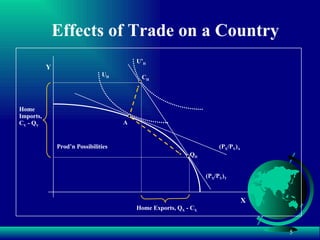
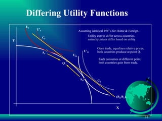
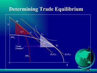
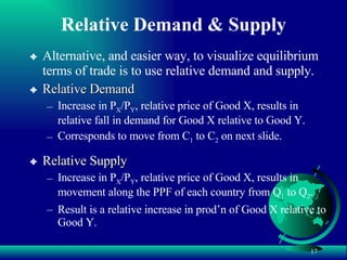
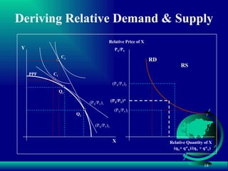
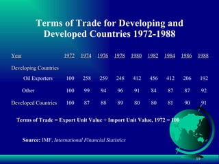
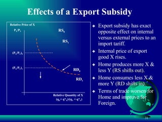
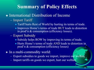
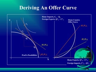
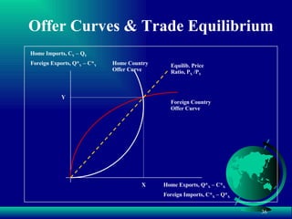
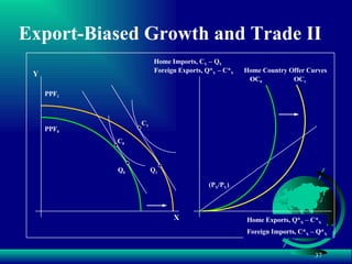
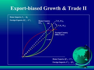
The document discusses the standard trade model and gains from trade. It introduces a 2x2x2 model with two countries producing two goods using two factors of production. Opening trade leads to gains for both countries as production and consumption move to new equilibrium points that exploit each country's comparative advantage. The terms of trade adjust to balance trade between the countries. Economic growth can impact a country's terms of trade depending on whether it is export- or import-biased. Government policies like tariffs, subsidies, and transfers also affect equilibrium terms of trade.

1. BA 187 – International Trade Standard Trade Model and Gains from Trade

2. Standard Trade Model Technology Two countries produce two goods, X & Y using two factors of production, labor, L and capital, K. (2 x 2 x 2 model) Prod’n function exhibits constant returns to scale, diminishing marginal returns to a factor. Economies have different endowments of the factors of prod’n. Tastes Economy’s preferences can be represented by community indifference curves. Assume away distortions like taxes, subsidies, imperfect competition.

3. Technology & Country PPF PPF: Shape shows diminishing marg. returns to factors of prod’n. Iso-Value Lines: For given set of relative prices, p x , shows prod’n points with equal value. Perfect Competition: Nation chooses highest iso-value line given its PPF. Y X Prod’n Possibilities Iso-value lines

4. Trade and Relative Prices Begin with country in autarkic equilibrium: relative price (P X /P Y ) A & consump/prod’n at point A. Opening country to trade changes relative price. Assume Home exports Good X, then new price will be steeper than in autarchy (P X /P Y ) T > (P X /P Y ) A . Home consumes at point C, produces at point Q Increases prod’n of Good X (which it exports). Increases consumption of Good Y (which it imports). As in Classical Model, opening trade leads to gains to both economies. You should be able to show that Foreign will also benefit, using a similar diagram.

5. (P X /P Y ) A Effects of Trade on a Country Y X Prod’n Possibilities A U H C H Q H (P X /P Y ) T U’ H Home Exports, Q X - C X Home Imports, C Y - Q Y

6. % Change in U.S. Employment Resulting from Foreign Trade, 1970-1980 Source: R.Z. Lawrence, Can America Compete? 19.9 Construction machinery 17.8 Engines & turbines 16.1 Office & computing machines 12.8 Aircraft & parts 8.0 Misc. machinery 5.7 Service industry machines -6.3 Apparel -6.3 Leather Products -7.8 Electrical components -11.1 Motor Vehicles & equipment -15.9 Footwear Percent Change Industry

7. Sources of Gains from Trade Can break a country’s gains from trade into two distinct parts. Gains from Exchange (Consumption Gains) Assume trade changes the relative price but the country continues to produce at the autarchy equilib. Point A. Nation still experiences a gain in welfare due to price change measured by move from point A to C 1 . Gains from Specialization (Production Gains) The change in relative price leads the country to change production from Point A to Point Q 1 . Nation experiences an additional gain in welfare due to prod’n specialization measured by move from point C 1 to C 2 . This is similar to the substitution/wealth effect analysis of a price change in microeconomics.

8. (P X /P Y ) 1 Sources of Gains from Trade Y X Prod’n Possibilities A 1 (P X /P Y ) 2 Q 2 C 2 C 1

9. Sources of the Basis for Trade

10. The Basis for Trade Mutual gains from trade arise in the Standard model of trade in essentially two ways: Differences in Production Possibilities PPF’s may differ across countries in ways that give rise to trade due to: Differences in Technology Differences in Factor Endowments Differences in Tastes Utility curves across countries can differ in ways that give rise to trade even when PPF’s are identical. Illustrate trade possibilities in these two situations

11. Differing Technology/Endowments Y X (P X /P Y ) * Opening trade changes relative prices Assuming identical utility function for Home & Foreign PPF H PPF F Home & Foreign PPF’s differ due to differences in technology or factor endowments. A H A F Autarky Equilibrium at A H and A F Q F Q H C * New equilib. consumption at C * . Each country has different prod’n ;point.

12. Differing Utility Functions Y X Assuming identical PPF’s for Home & Foreign. A H U H C H U’ H A F U F Utility curves differ across countries, autarchy prices differ based on utility. Q * (P X /P Y ) * Open trade, equalizes relative prices, both countries produce at point Q. C F U’ F Each consumes at different point, both countries gain from trade.

13. Revealed Comparative Advantage Composition of Exports & Imports of the U.S., Europe, and Japan in 1990 Source: GATT, International Trade, 1991-1992 2.2 23.3 5.5 23.1 (95.9) 0.4 0.6 (2.5) Exports Japan % of Total 5.5 4.8 6.5 3.1 (42.6) 24.5 14.5 (54.8) Imports 6.3 6.1 12.0 11.7 (79.7) 3.7 10.4 (18.4) Exports Europe % of Total 6.8 8.2 10.0 9.2 (71.0) 8.8 10.7 (26.8) Imports 6.5 1.9 Textiles 12.3 13.1 Telecomm 4.6 10.0 Chemicals 15.2 9.0 Autos (75.5) (73.9) Manufactures 13.3 3.1 Fuel 5.8 10.8 Food (24.1) (21.2) Commodities Imports Exports U.S. % of Total

14. Determining Trade Equilibrium

15. Trade Equilibrium In equilibrium, terms of trade adjust to ensure balanced trade between the two countries. Current account = 0 in Standard Trade Model equilib. Can illustrate trade equilibrium using diagram of PPF’s and utility curves for the two countries. Both PPF’s & utility curves differ across countries initially. Autarchy relative prices differ, leading to potential gains from trade. Trade equalizes relative prices across countries. In equilibrium, this relative price adjusts to make trade triangles for each country identical, i.e. balanced trade.

16. Determining Trade Equilibrium Y X PPF H PPF F C F (P X /P Y ) * “ Trade Triangles” A H (P X /P Y ) * Q H C H A F C F (P X /P Y ) * Q F

17. Relative Demand & Supply Alternative, and easier way, to visualize equilibrium terms of trade is to use relative demand and supply. Relative Demand Increase in P X /P Y , relative price of Good X, results in relative fall in demand for Good X relative to Good Y. Corresponds to move from C 1 to C 2 on next slide. Relative Supply Increase in P X /P Y , relative price of Good X, results in movement along the PPF of each country from Q 1 to Q 2 . Result is a relative increase in prod’n of Good X relative to Good Y.

18. Deriving Relative Demand & Supply Y X PPF (P X /P Y ) 1 Q 1 C 1 P X /P Y Relative Price of X (q X + q* X )/(q Y + q* Y ) Relative Quantity of X (P X /P Y ) 2 Q 2 C 2 RD RS (P X /P Y ) 2 (P X /P Y ) 1 (P X /P Y )*

19. Terms of Trade for Developing and Developed Countries 1972-1988 Terms of Trade = Export Unit Value ÷ Import Unit Value, 1972 = 100 Source: IMF, International Financial Statistics 91 92 192 1988 90 87 206 1986 81 87 412 1984 80 84 456 1982 80 91 412 1980 89 96 248 1978 88 94 259 1976 87 99 258 1974 100 100 100 1972 Developed Countries Other Oil Exporters Developing Countries Year

20. Growth & Trade Equilibrium

21. Economic Growth & Trade How does economic growth both in our country & in the rest of the world affect trade? Ambiguity at “common sense” level Our growth means better able to export to world but May mean receive lower prices for our exports. Similar considerations for growth in rest of world. We look only at effects of growth on trade, particularly a country’s terms-of-trade. Our economic growth increases our GDP directly but look at whether effect through trade adds or subtracts from this benefit of growth. Similarly growth in another nation has no direct effect on us but may benefit or hurt us through effect on trade.

22. Growth and a Nation’s PPF Economic growth shifts out a nation’s PPF. Trade effects occur because growth often biased, shifts PPF out more in one good than the other. Export-biased Growth Growth that expands a nation’s PPF more towards its export good. Import-biased Growth Growth that expands a nation’s PPF more towards its import good.

23. Export-Biased Growth and Trade Y X PPF 0 Q 0 RD 0 RS 0 (P X /P Y ) 0 P X /P Y Relative Price of X (q X + q* X )/(q Y + q* Y ) Relative Quantity of X PPF 1 Q 1 RS 1 (P X /P Y ) 1

24. Import-Biased Growth and Trade Y X PPF 0 Q 0 RD 0 RS 0 (P X /P Y ) 0 P X /P Y Relative Price of X (q X + q* X )/(q Y + q* Y ) Relative Quantity of X PPF 1 RS 1 (P X /P Y ) 1 Q 1

25. Economic Growth & Welfare Export-biased growth tends to worsen a nation’s terms of trade benefiting the rest of the world. Import-biased growth tends to improve a nation’s terms of trade at the rest of the world’s expense. Immiserizing Growth 1950’s belief that export-biased growth could worsen terms of trade so much that nation worse off than if had not grown at all. Requires extreme conditions unlikely to hold in real world (large shift, steep RS & RD curves)

26. Trade Policy & Equilibrium

27. Trade Policy & Equilibrium Look at effects of three types of gov’t policies on terms of trade equilibrium. International Income Transfers Pure income transfers (aid) or short run effects of changes in international lending. Import Tariffs Taxes levied on nation’s imports Export Subsidies Payments given to domestic producers of export goods.

28. International Income Transfers RS 0 (q X + q* X )/(q Y + q* Y ) Relative Quantity of X P X /P Y Relative Price of X (P X /P Y ) 0 RD 0 Income transfer from Home to Foreign. Home expenditure falls, Foreign expenditure rises. Net result for RD depends on differences in marg. prop. to spend on Good X between Home & Foreign. Transfer shifts RD back if donor has higher mps on its export than recipient. Donor’s terms of trade worsen. RD 1 (P X /P Y ) 1

29. Import Tariffs & Terms of Trade Both tariffs & subsidies drive a wedge between prices of goods internationally (external prices) & domestically (internal prices). Tariff Makes imported goods more expensive within a nation than they are outside. This has two effects within nation: Home producers face lower relative price of Good X & so produce less X and more Y. (RS falls) Home consumers demand less Y and more X. (RD rises) Home’s terms of trade improve at expense of Foreign. Size of effect depends on how large Home is relative to ROW. If country is small then little impact on world RD and RS so correspondingly small effect on terms of trade

30. Effects of a Import Tariff RD 0 RS 0 (P X /P Y ) 0 (q X + q* X )/(q Y + q* Y ) Relative Quantity of X P X /P Y Relative Price of X Import tariff decreases internal relative price of export good X vs. good Y. Internal price of export good X falls. Home produces less X & more Y (RS shifts in). Home consumes less X & more Y (RD shifts out). Terms of trade improve for Home and worsen for Foreign. (P X /P Y ) 1 RD 1 RS 1

31. Effects of a Export Subsidy (q X + q* X )/(q Y + q* Y ) Relative Quantity of X P X /P Y Relative Price of X (P X /P Y ) 0 RD 0 RS 0 Export subsidy has exact opposite effect on internal versus external prices to an import tariff. Internal price of export good X rises. Home produces more X & less Y (RS shifts out). Home consumes less X & more Y (RD shifts in). Terms of trade worsen for Home and improve for Foreign. (P X /P Y ) 1 RS 1 RD 1

32. Summary of Policy Effects International Distribution of Income Import Tariff Tariff hurts Rest of World by hurting its terms of trade. Improves Home’s terms of trade BUT leads to distortion in prod’n & consumption (efficiency losses). Export Subsidy Subsidy helps ROW by improving its terms of trade. Hurts Home’s terms of trade AND leads to distortion in prod’n & consumption (efficiency losses) In a multi-commodity world: Export subsidies to goods we import, improve our welfare Import tariffs on goods we export, hurt our welfare.

33. Alternative Method to Determine Trade Equilibrium

34. Offer Curves and Trade Equilib. Offer Curve analysis focuses explicitly on a country’s exports and imports at any terms of trade. Use PPF/Utility function diagram to generate difference between consumption and prod’n for each good at any relative price (its trade triangle at each relative price). Offer Curve Diagram summarizes these trade triangles with relative price equal to slope of ray from origin. Can construct an Offer Curve for each country. Point at which they cross is where trade is balanced, i.e. trade triangles are equal. Can use to analyze effects of growth or trade policy as alternative to relative demand/supply approach.

35. Deriving An Offer Curve Y X Prod’n Possibilities (P X /P Y ) 1 Q 1 C 1 Foreign Exports, Q* Y – C* Y Home Imports, C Y – Q Y Foreign Imports, C* X – Q* X Home Exports, Q* X – C* X Q 2 (P X /P Y ) 2 C 2 (P X /P Y ) 2 (P X /P Y ) 1 Home Country Offer Curve

36. Offer Curves & Trade Equilibrium Foreign Exports, Q* Y – C* Y Home Imports, C Y – Q Y Foreign Imports, C* X – Q* X Home Exports, Q* X – C* X Foreign Country Offer Curve Home Country Offer Curve Equilib. Price Ratio, P X /P Y X Y

37. PPF 1 Q 1 Export-Biased Growth and Trade II Y X PPF 0 Q 0 Foreign Exports, Q* Y – C* Y Home Imports, C Y – Q Y Foreign Imports, C* X – Q* X Home Exports, Q* X – C* X (P X /P Y ) OC 0 C 0 C 1 OC 1 Home Country Offer Curves

38. Export-biased Growth & Trade II Home Country OC 0 Foreign Exports, Q* Y – C* Y Home Imports, C Y – Q Y Foreign Imports, C* X – Q* X Home Exports, Q* X – C* X ( P X /P Y ) 0 ( P X /P Y ) 1 OC 1 Foreign Country Offer Curve