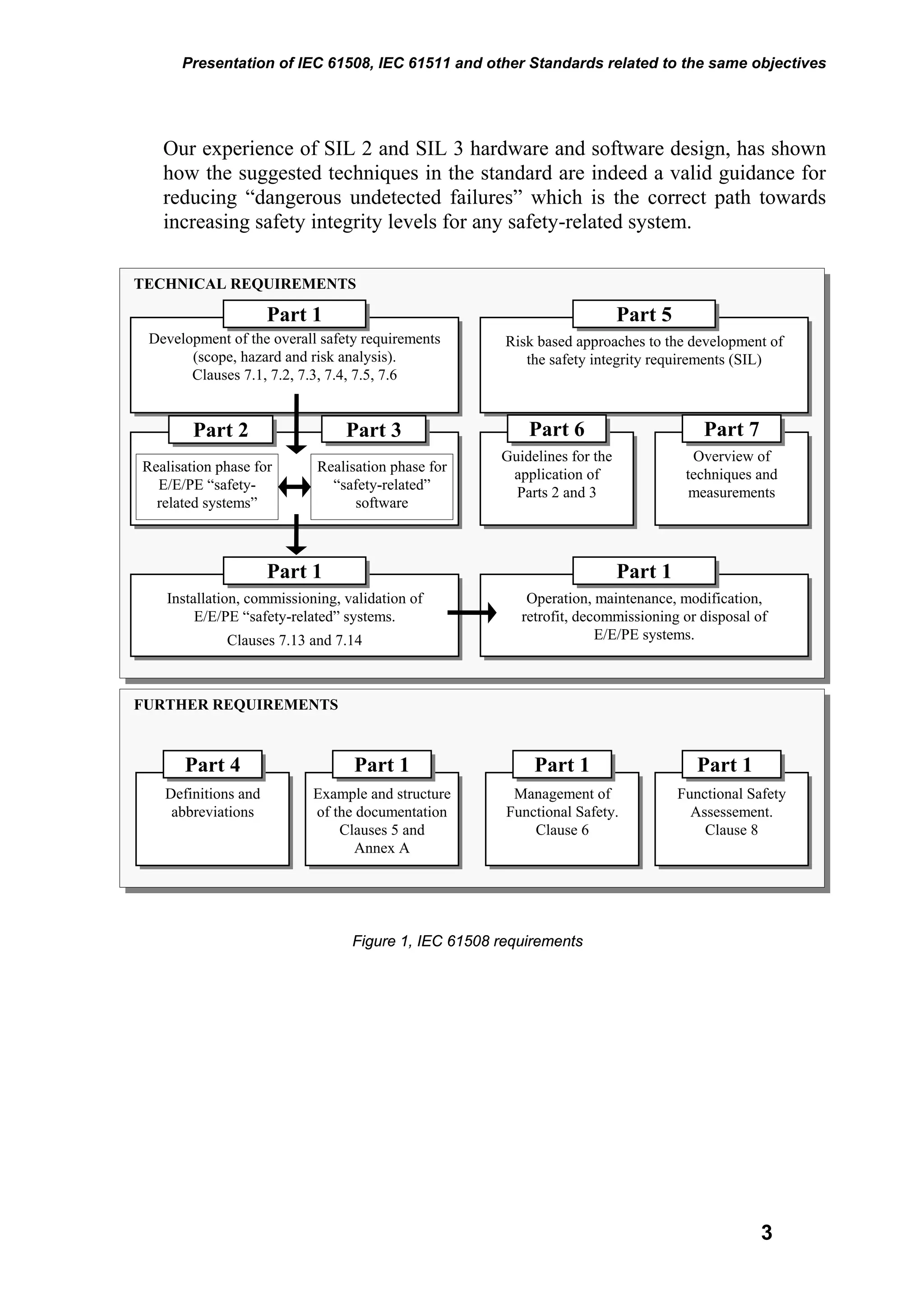
This document introduces several important safety standards, including IEC 61508 and IEC 61511. IEC 61508 provides a framework for functional safety of electrical, electronic, and programmable electronic systems. It aims to standardize the design of safety instrumented systems and evaluate their effectiveness through requirements for documentation, risk analysis, and other lifecycle processes. IEC 61511 applies IEC 61508 specifically to safety instrumented systems for process industry. Other referenced standards provide complementary guidelines for hazard analysis, risk assessment, and specific applications. The introduction of these international standards aims to improve safety system design and more accurately define risk through a scientific, technical, and consistent approach.

1. SAFETY
INSTRUMENTED
SYSTEMS
Plant Engineering and Maintenance
according to IEC 61508 and IEC 61511 Standards
• Safety Integrity Levels
• Reliability and Probability of Failure on Demand
• Redundant System Architectures
• Risk Reduction
• IEC 61508 and IEC 61511 compendiums
SIL MANUAL
3rd
Edition

2. SAFETY INSTRUMENTED SYSTEMS
Manual for
Plant Engineering
and Maintenance
With reference to
IEC 61508 Standard for Functional Safety of
Electrical / Electronic / Programmable Electronic
Safety-Related Systems
and
IEC 61511 Safety Instrumented Systems for the
Process Industry
3rd
Edition

3. Authors
Abbamonte Basilio
Software Development and Quality Assurance Manager G.M. International
Francesco Landrini
IT Manager G.M. International
Giorgio Novelli
Technical Director G.M. International
Glisente Landrini
President and Commercial Director G.M. International
Massimo Baldrighi
R&D Project Manager G.M. International

4. Why this manual was written
G.M. International designs, manufactures and sells SIL2 and SIL 3 certified
Intrinsically Safe Interfaces for use in Hazardous Locations; these products
are intended to prevent accidents before they occur, thus reducing risk and
enhancing safety in a very wide variety of applications.
This manual is a practical aid for the analysis, installation and maintenance of
safety instrumented systems and associated components and will hopefully
serve as a guide for understanding procedures and transposing them into
practice.
It represents our effort to share the results we have come to after many years
of research and field experience, with anyone willing to approach Safety
Related Systems.
Who this manual is for
This manual is not intended for safety reliability specialists, but for the
thousands of professionals employed in process industries who work with
safety instrumented systems and who are expected to follow the appropriate
industry standards.
Aren’t the standards alone enough? The answer depends upon the knowledge
and experience of the individual and the company.
The growing demand for experts in a critical sector like functional safety,
underlies the urgency of a greater awareness and comprehension of all
subjects presented herein.

5. Index
Index
Authors ................................................................................................... 3
Why this manual was written......................................................................... 4
Who this manual is for ................................................................................... 4
Index .................................................................................................... I
Chapter 1 Presentation of IEC 61508, IEC 61511 and other safety
related standards..................................................................... 1
1.1 Scope of the IEC 61508 ....................................................................................4
1.1.1 Safety ...........................................................................................................5
1.1.2 IEC 61508: Brief description. .......................................................................7
1.2 Other safety-related standards........................................................................10
1.2.1 HSE- PES...................................................................................................10
1.2.2 DIN (V) 19250 ............................................................................................10
1.2.3 AIChE - CCPS............................................................................................11
1.2.4 ISA-SP84.01 - 1996 ...................................................................................11
1.2.5 API RTP 556 ..............................................................................................12
1.2.6 NFPA 85.....................................................................................................12
1.2.7 IEC 61511 – 2004 (ANSI/ISA-84.00.01-2004)...........................................12
1.2.8 API RP 14C................................................................................................13
1.2.9 Risk of relevant accidents, in EEC and Italian Standards .........................13
Chapter 2 Prevention and mitigation layers for hazardous events .... 15
2.1 Plants and processes in their environmental context ....................................18
2.2 Process Control System..................................................................................20
2.3 Alarm system...................................................................................................21
2.4 Emergency Shutdown system.........................................................................23
2.5 Physical protection and release devices.........................................................24
2.6 Physical protections and containment systems ..............................................26
2.7 Physical protections and dispersion systems .................................................27
2.8 Physical protections and Fire & Gas neutralizing systems.............................27
2.9 Internal emergency plan (evacuation procedures) ........................................29
I

6. Index
2.10 External emergency plan (evacuation procedures) .......................................29
Chapter 3 Basic concepts for a better comprehension of safety
standards ............................................................................... 31
3.1 Reliability and Unreliability ..............................................................................31
3.1.1 Reliability ....................................................................................................31
3.1.2 Unreliability.................................................................................................34
3.2 Availability and unavailability...........................................................................36
3.2.1 Ambiguity of the term “availability” .............................................................38
3.2.2 Achievable Availability................................................................................41
3.2.3 Operational Availability...............................................................................41
3.3 MTTF, MTTR, MTBF and their relations .........................................................42
3.4 Failure Rate.....................................................................................................45
3.4.1 Components with constant failure rate.......................................................47
3.4.2 Failure rate Categories...............................................................................48
3.4.3 Dependent, or common cause, failures .....................................................50
3.4.4 Common cause failures and Beta factor....................................................51
3.5 Safety analysis for SIL level selection: Modeling methods ............................52
3.5.1 Reliability block diagrams...........................................................................52
3.5.2 Fault tree analysis ......................................................................................54
3.5.3 Markov diagrams........................................................................................59
Chapter 4 Consequence Analysis of relevant accidents involving
chemical substances ............................................................ 71
4.1 Analysis of risks from the release of chemical substances.............................71
4.2 Flammability effects.........................................................................................76
4.2.1 Pool fire ......................................................................................................76
4.2.2 Jet fire.........................................................................................................78
4.2.3 Flash fire.....................................................................................................79
4.2.4 Fireball / BLEVE.........................................................................................80
4.2.5 Explosion effects ........................................................................................81
4.3 Toxic hazard: Dispersion modeling.................................................................84
Chapter 5 Safety Instrumented Systems (SIS)..................................... 87
5.1 Introduction......................................................................................................87
5.2 Safety requirements ........................................................................................89
5.3 Average Probability of Failure on Demand (PFDavg), Safety Integrity Levels
(SIL).................................................................................................................91
5.4 System architectures.......................................................................................98
5.4.1 Introduction.................................................................................................98
II

7. Index
5.4.2 Common cause factor (β) and PFDavg for redundant architectures.......102
5.4.3 1oo1 system architecture.........................................................................104
5.4.4 1oo2 architecture .....................................................................................112
5.4.5 2oo3 system architecture.........................................................................118
5.4.6 Comparison between system architectures.............................................122
5.5 Summary of simplified equations ..................................................................124
5.5.1 Influence of time interval and duration of periodic tests, on PFDavg, for
redundant equal components ..................................................................126
5.5.2 Application exercises using simplified equations.....................................126
5.6 Use of valves in Safety Instrumented Systems.............................................128
5.6.1 Bypass examples and possibilities of on-line periodic proof testing for
SIS shutdown valves, or other field devices used in 1oo1 system
architecture ..............................................................................................128
5.6.2 Partial Stroking Test (PST) for valves......................................................130
5.6.3 Full Stroke Test of valves (FST) ..............................................................132
5.7 SIS Conceptual Design ................................................................................133
5.7.1 Conceptual Design Requirements ...........................................................134
5.8 Lifecycles cost analysis.................................................................................136
5.9 Conceptual Design and SIL Level.................................................................137
Chapter 6 IEC 61508: Fundamental concepts .................................... 139
6.1 Overall safety lifecycle...................................................................................139
6.2 Safety Integrity Levels...................................................................................141
6.3 Part “1”: General requirements .....................................................................142
6.3.1 Scope .......................................................................................................142
6.3.2 Compliance ..............................................................................................143
6.3.3 Documentation (Clause 5) .......................................................................144
6.3.4 Management of Functional Safety (Clause 6) .........................................145
6.3.5 Overall Safety Lifecycle Requirements (Clause 7) ..................................146
6.3.6 HSE Findings ...........................................................................................147
6.3.7 The concept of safety lifecycle in IEC 61508...........................................148
6.3.8 Functional Safety Assessment (Clause 8)...............................................151
6.3.9 Example documentation structure (Annex A) ..........................................152
6.3.10 Competence of persons (Annex B)..........................................................153
6.4 Part “2”: Hardware Requirements .................................................................154
6.4.1 Control of Failure during Operation (Annex A) ........................................157
6.4.2 Avoidance of Systematic Failures during different phases of the Lifecycle
(Annex B) .................................................................................................157
6.4.3 Diagnostic Coverage and Safe Failure Fraction (Annex C).....................158
III

8. Index
6.5 Part “3”: Software requirements ....................................................................159
6.5.1 Software Functional Safety Plan (Clause 6) ............................................159
6.5.2 Software Safety Lifecycles (Clause 7) .....................................................161
6.5.3 Software Safety Requirements Specification (Clause 7.2).....................163
6.5.4 Software safety validation planning (Clause 7.3).....................................163
6.5.5 Software design and development (Clause 7.4)......................................164
6.5.6 Integration and testing (Clause 7.5).........................................................165
6.5.7 Software safety validation (Clause 7.7) ...................................................165
6.5.8 Operation and modification (Clause 7.6 and 7.8) ....................................166
6.5.9 Software verification (Clause 7.9) ............................................................167
6.5.10 Software Functional Safety Assessment (Clause 8)................................167
6.5.11 Guide to the selection of techniques and measures (Annexes “A” and
“B”)............................................................................................................168
6.6 Part “4”: Definitions and abbreviations..........................................................169
6.7 Part “5”: Safety Integrity Level determination................................................169
6.7.1 Risk Reduction – General concepts.........................................................169
6.7.2 Risk and safety integrity: general concepts (Annex A) ...........................173
6.7.3 ALARP and tolerable risk concepts (Annex “B”)......................................174
6.7.4 Tolerable Risk decisions based on financial considerations ..................176
6.7.5 Quantitative method for SIL determination (Annex “C”)..........................179
6.7.6 Qualitative method: Risk graph (Annex “D”) ............................................182
6.7.7 Determination of the SIL level: qualitative method, Hazardous event
severity matrix (Annex “E”).......................................................................185
6.7.8 Layer of Protection Analysis (LOPA)........................................................185
6.8 Part “6”: Guidelines in the application of Parts 2 and 3................................189
6.8.1 Application of Parts 2 and 3 (Annex “A”)..................................................189
6.8.2 Example technique for evaluating probabilities of hardware failure
(Annex “B”) ...............................................................................................189
6.8.3 Diagnostic Coverage calculation and Safe Failure Fraction: Worked
example (Annex “C”) ................................................................................189
6.8.4 Methodology to quantify the effect of the common failures of the
hardware in the E/E/PE multichannel systems (Enclosure “D”)...............193
6.8.5 Applicative example of the integrity software table of Part 3 (Enclosure
“E”)............................................................................................................193
6.9 Part 7: Overview of techniques and measures .............................................194
6.9.1 Overview of techniques and measures for E/E/PES: control of random
hardware failures (Annex “A”) ..................................................................194
6.9.2 Overview of techniques and measures for E/E/PES: avoidance of
systematic failures (Annex “B”) ................................................................194
IV

9. Index
6.9.3 Overview of techniques and measures for achieving software safety
integrity (Annex “C”).................................................................................194
6.9.4 A probabilistic approach to determining software safety integrity for pre-
developed software (Annex “D”) .............................................................194
Chapter 7 IEC 61511 Safety Instrumented Systems for process
industry................................................................................. 195
7.1 Part 1: Framework, definitions, system, hardware and software
requirements .................................................................................................196
7.2 Part 2: Guidelines in the application of IEC 61511 ......................................198
7.3 Part 3: Guidelines in the application of hazard and risk analysis ................199
Chapter 8 Proven-in-use assessment ................................................. 201
8.1 Defining the term “proven-in-use” according IEC 61508-7 ...........................201
8.2 “Proven-in-use” requirements according to IEC 61511-1 .............................202
8.3 Required information for a proven-in-use proof of a sub-system .................203
Chapter 9 Functional safety manual.................................................... 205
9.1 Requirements................................................................................................205
9.2 Example ........................................................................................................207
Chapter 10 SIS design checklists.......................................................... 209
10.1 Management Requirements..........................................................................210
10.2 Safety Requirements Specification ...............................................................211
10.3 Conceptual SIS Design .................................................................................212
10.4 Detailed SIS Design ......................................................................................213
10.5 Power & Grounding.......................................................................................214
10.6 Field Devices.................................................................................................215
10.7 Operator Interface .........................................................................................216
10.8 Maintenance/Engineering Interface ..............................................................217
10.9 Communications............................................................................................217
10.10 Hardware Specifications ...............................................................................218
10.11 Hardware Manufacture..................................................................................219
10.12 SIF Components ...........................................................................................220
10.13 Application Logic Requirements....................................................................222
10.14 Embedded (Vendor) Software ......................................................................223
10.15 Software Coding............................................................................................224
10.16 Factory Test ..................................................................................................225
10.17 Installation & Commissioning........................................................................226
10.18 Operations & Maintenance............................................................................228
V

10. Index
VI
10.19 Testing...........................................................................................................230
10.20 Management of Changes..............................................................................231
10.21 Decommissioning ..........................................................................................232
Index of Words............................................................................................ 233
Index of Figures.......................................................................................... 236
Index of Tables ........................................................................................... 239
Reference .............................................................................................. 241
Denial of responsibility .............................................................................. 242

11. Presentation of IEC 61508, IEC 61511 and other Standards related to the same objectives
Chapter 1 Presentation of IEC 61508, IEC 61511
and other safety related standards
Safety-related systems serve the function of protecting equipments and
industrial processes where danger may occur in case of failure.
These systems are not part of the process control system since their purpose is
to bring the plant to a safe state in case of malfunctioning.
Until a few years ago these systems, for example ESD systems (Emergency
Shut-Down), were being designed in compliance with the respective standards
in force in the different countries, with no reference to a general normative.
This condition is now changing with the introduction of the
IEC 61508 and IEC 61511.
With these Standards, the most important benefits for the final user are:
‰ A more technical and scientific method in formulating requirements, and
specifications in designing process.
‰ A more accurate definition of risk.
‰ A more valid designing of safety-related system.
‰ An easier and wider demonstration of safety-related system’s
effectiveness.
‰ A far more cost-effective implementation of safety-related system.
‰ An easier evaluation and effectiveness of maintenance operations.
The number of manufacturers of equipments complying with this standard is
expected to grow. Information provided by the manufacturers allow the
integration of their products into safety-related systems.
IEC 61508 is an international standard for the “functional safety” of electrical,
electronic, and programmable electronics equipment.
At present, in Europe, EN 61508 has been issued but not yet acknowledged as
European Directive.
This standard started in the mid 1980s when the International Electrotechnical
Committee Advisory Committee of Safety (IEC ACOS) set up a task force to
consider standardization issues raised by the use of a programmable electronic
system (PES).
At that time, many regulatory bodies forbade the use of any software-based
equipment in safety critical applications.
1

12. Presentation of IEC 61508, IEC 61511 and other Standards related to the same objectives
Work began within IEC SC65A/Working Group 10 on a standard for PES
used in safety-related systems. The group merged with Working Group 9
where a standard on software safety was in progress.
The combined group treated safety as a system issue.
IEC 61508 is divided into seven parts.
The first three are required for compliance (normative), the others are
supporting information (informative) which provide further guidance
information.
‰ Part 1: General requirements. (Normative)
‰ Part 2: Requirements for electrical/electronic/programmable
electronic safety-related systems. (Normative)
‰ Part 3: Software requirements. (Normative)
‰ Part 4: Definitions and abbreviations. (Informative)
‰ Part 5: Examples of methods for the determination of safety integrity
levels. (Informative)
‰ Part 6: Guidelines on the application of Parts 2 and 3. (Informative)
‰ Part 7: Overview of techniques and measures. (Informative)
Parts 1, 3, 4 and 5 were approved in 1998. Parts 2, 6 and 7 were approved in
February 2000. The relationship between technical requirements presented in
parts 1, 2 and 3 and the supporting information in parts 4 through 7 is shown
in Figure 1, in the following page.
Although the standard has been criticized for the “extensive” documentation
requirements and use of unproven “statistical” techniques, in many industries
it represents a great step forward.
The standard focuses attention on risk-based safety-related systems design,
which should result in far more cost-effective implementations.
It also requires the attention to details that is vital to any safe system design.
Because of these features and the large degree of international acceptance for
a single set of documents, many consider the standard to be major advance for
the technical world.
2

13. Presentation of IEC 61508, IEC 61511 and other Standards related to the same objectives
Our experience of SIL 2 and SIL 3 hardware and software design, has shown
how the suggested techniques in the standard are indeed a valid guidance for
reducing “dangerous undetected failures” which is the correct path towards
increasing safety integrity levels for any safety-related system.
TECHNICAL REQUIREMENTS
Figure 1, IEC 61508 requirements
Development of the overall safety requirements
(scope, hazard and risk analysis).
Clauses 7.1, 7.2, 7.3, 7.4, 7.5, 7.6
Part 1
Risk based approaches to the development of
the safety integrity requirements (SIL)
Part 5
Part 2 Part 3
Realisation phase for
E/E/PE “safety-
related systems”
Realisation phase for
“safety-related”
software
Guidelines for the
application of
Parts 2 and 3
Part 6
Overview of
techniques and
measurements
Part 7
Installation, commissioning, validation of
E/E/PE “safety-related” systems.
Clauses 7.13 and 7.14
Part 1
Operation, maintenance, modification,
retrofit, decommissioning or disposal of
E/E/PE systems.
Part 1
FURTHER REQUIREMENTS
Definitions and
abbreviations
Part 4
Example and structure
of the documentation
Clauses 5 and
Annex A
Part 1
Management of
Functional Safety.
Clause 6
Part 1 Part 1
Functional Safety
Assessement.
Clause 8
3

14. Presentation of IEC 61508, IEC 61511 and other Standards related to the same objectives
1.1 Scope of the IEC 61508
There is a primary safety, (which deals with risks, as electric discharges
generated by an electric equipment), a functional safety (to which this
standard specifically refers), which depends on the measures of risk reduction
adopted in the system under control, or EUC (Equipment Under Control),
and a derived safety which deals with the indirect consequences of an EUC,
which does not perform as expected, for example providing a drug with a
wrong recipe which might kill instead of healing.
However, the principles of this standard can also be generally applied to other
aspects of safety not specifically referring to its functionality.
IEC 61508 is one of the main publications, on safety matters, of IEC
(International Electrotechnical Commission). As such, it is a document which
involves many industries and applications.
It involves, for example, the PED directive (Pressured Equipment Directive)
and the protection method “b” for non electrical equipments of ATEX
(mechanic), as well as the new normative (not yet approved) EN 50495
(Safety devices required for safe functioning of equipment with respect to
explosion risks), in which, for the first time in ATEX standard, functional
safety integrity levels are used (SIL levels) as protection system.
The main purpose of IEC 61508 is to provide the basis for the preparation of
specific safety standards for plant and industrial sectors.
A second scope of the standard is to help the development of safety-related
systems E/E/PE (Electrical/Electronic/Programmable Electronic) where
specific standards do not exist.
Starting from 2002, two new specific standards directly referring to IEC
61508 were introduced: IEC 61511 for process control industries and IEC
62061 (EN 954) Safety of Machinery.
IEC 61508 covers safety-related systems when one or more of such systems
incorporate electrical/electronic/programmable electronic devices.
These devices can include anything from electrical relays and switches to
Programmable Logic Controllers (PLCs) and all the way up to complicated
computer-driven overall safety systems.
The standard specifically covers possible hazards created when failures of
safety functions performed by E/E/PE safety-related systems occur.
The overall program to insure that a safety-related E/E/PE system brings
about a safe state, when called upon to do so, is defined as “functional
safety”.
4

15. Presentation of IEC 61508, IEC 61511 and other Standards related to the same objectives
IEC 61508 does not cover safety issues like electric shock, hazardous falls,
long-term exposure to a toxic substance, etc.; these issues are covered by
other standards like ATEX or similar.
IEC 61508 also does not cover low safety E/E/PE systems where a single
E/E/PE system is capable of providing the necessary risk reduction and the
required safety integrity level of the E/E/PE system is less than SIL 1.
IEC 61508 is concerned with the E/E/PE safety-related systems whose failure
could affect the safety of persons and/or the environment. However, it is
recognized that the methods of IEC 61508 also may be applied to business
loss and asset protection cases.
Note:
Difficulties may be found in the first reading of the standard, which requires
attention and undertaking, attitudes not always available after a long and
exhausting working day.
Starting from Part 4 (Definitions and abbreviations) can be very useful for the
comprehension of the whole standard.
1.1.1 Safety
When considering an industrial process, it is recognized that there is an
inherent risk of operation. Sometimes things do go wrong.
The standard defines Safety as “freedom from unacceptable risk of harm”.
IEC 61508 goes on defining the level of safety as “a level of how far safety is
to be pursued in a given context, assessed by reference to an acceptable risk,
based on current values of society”.
When evaluating safety, the frequency of an accident and the consequences
(costs) of an accident are both taken into consideration.
Risk is defined as the probable rate of occurrence of a hazard causing harm
and its degree of severity. Thus, risk evaluation includes a combination of
frequency and cost.
Generally, risk (R) is the result of multiplication between the frequency of
accidents (F) and their consequences (C).
R = F×C
5

16. Presentation of IEC 61508, IEC 61511 and other Standards related to the same objectives
Example:
If the consequences of an accident are estimated to be 100’000’000 $ and the
frequency of the accident is estimated to be once every 10 years (probability
of an accident is 0.1 for a time interval of one year).
The inherent risk is stated to be 10’000’000 $ per year (10 = 0,1 x 100).
Note that the concept of inherent risk refers to a context with no protections.
The present industrial world, with the necessity of larger productions and
lower costs, has certainly increased the probability of severe accidents.
Beyond damages to persons and environment, created by an accident, legal
expenses costs, fines, commercial losses caused by plant shutdown and by bad
reputation, have to be considered. Risk reduction is therefore mandatory.
Note:
From an ethical point of view, it could be objected that “damages to things” or
“death of one or more persons”, as mentioned in IEC 61508, should not be
quantified only in economic terms. Although, beyond this being the regular
procedure for insurance companies, it responds to a normative criterion of
uniformity to generalize the methods of calculation.
The evaluation of human resources, as well as human factors is not a subject
of this standard.
Following are the first 6 definitions available in Part 4 of the standard:
‰ Hazard
Potential source of harm.
Note: The term includes danger to persons arising within a short time scale
(e.g. fire and explosion) and also those that have a long-term effect on a
person’s health (e.g. release of a toxic substance).
‰ Hazardous situation
Circumstance in which a person is exposed to hazard/s
‰ Hazardous event
Hazardous situation which resolves in a harm.
‰ Risk
Combination of the probability of occurrence of harm and its severity.
‰ Tolerable risk
Accepatble Risk in a given context based on the current values of society.
‰ Residual risk
Risk remaining after protective measurements have been taken.
6

17. Presentation of IEC 61508, IEC 61511 and other Standards related to the same objectives
1.1.2 IEC 61508: Brief description.
Part 1
Part 1 covers basic requirements of the standard and provides a detailed
presentation of the safety lifecycle. This section is considered to be the most
important, as it provides overall requirements for documentation, compliance,
management of functional safety, and functional safety assessment.
Three annexes provide examples of documentation structure (Annex A), a
personnel competency evaluation (Annex B), and a bibliography (Annex C).
Part 2
Part 2 covers the hardware requirements for safety-related systems.
Many consider this part, along with Part 3, to be the key area for those
developing products for the safety market.
Part 2 is written with respect to the entire system but many requirements are
directly applicable to safety-related hardware products development.
It covers a detailed safety lifecycle for hardware as well as specific aspects of
assessing functional safety for the hardware and has also detailed
requirements for techniques to deal with “control of failures during operation”
in Annex A (required for compliance).
This annex covers hardware fault tolerance, diagnostic capability
requirements and limitations, and systematic safety integrity issues for
hardware.
Annex B (required for compliance) contains a listing of “techniques and
measures” for “avoidance of systematic failures during different phases of the
lifecycle”. This covers design, analysis, and review procedures required by
the standard.
Annex C (required for compliance) discusses the calculation of the diagnostic
coverage factor (what fraction of failures are identified by the hardware) and
the safe failure fraction (what fraction of failures lead to a safe rather than
hazardous state).
Part 3
Part 3 covers software requirements for IEC 61508. It applies to any software
used in or to develop a safety-related system. This software is specifically
named safety-related. This part provides details of the software safety
lifecycle, a process to be used during development.
Annex A (required for compliance) provides a listing of “techniques and
measures” used for software development where different development
techniques are chosen depending on the SIL level of the software.
7

18. Presentation of IEC 61508, IEC 61511 and other Standards related to the same objectives
Annex B (required for compliance) has nine detailed tables of design, coding
standards, analysis and testing techniques that are to be used in the
safety-related software development, depending on the SIL level and, in some
cases, the choice of the development team.
Part 4
Part 4 contains definitions and abbreviations used throughout all parts of the
standard. This section is extremely useful both to those new to the standard
and to those already familiar with it, as a reference to the precise meaning of
terms in the standard.
Part 5
Part 5 includes informative Annexes A through E which contain discussions
and example methods for risk, safety integrity, tolerable risk, and SIL level
selection. It presents several techniques of SIL selection including both
quantitative and qualitative methods. The quantitative method in Annex C is
based on calculating the frequency of the hazardous event from failure rate
data or appropriate predictive methods combined with an assessment of the
magnitude of the consequence compared to the level of risk that can be
tolerated in the given situation.
The qualitative risk graph and severity matrixes essentially address the same
frequency and magnitude components, only with general categories rather
than numbers before comparing the situation with the tolerable risk level.
Part 6
Part 6 provides guidelines on the application of Part 2 and 3 via informative
Annexes A through E. Annex A gives a brief overview of Part 2 and 3 as well
as example flowcharts of detailed procedures to help with implementation.
Annex B provides example techniques for calculating probabilities of failure
for the safety-related system with tables of calculation results.
Equations that approximate various example architectures are presented,
although reliability block diagrams are used and these can be confusing in
multiple failure mode situations.
Annex C shows detailed calculation of diagnostic coverage factor based on
FMEDA (Failure Modes, Effects, and Diagnostics Analysis) techniques.
Annex D shows a method for estimating the effect of common cause modes of
failure (beta factor) in redundant hardware architecture.
This method lists relevant parameters and provides a method of calculation.
Annex E shows examples applying the software integrity level table of part 3
for two different safety software cases.
8

19. Presentation of IEC 61508, IEC 61511 and other Standards related to the same objectives
Part 7
Part 7 contains important information for those doing product development
work on equipment to be certified per IEC 61508.
Annex A addresses control of random hardware failures. It contains a
reasonable level of details on various methods and techniques useful for
preventing or maintaining safety in the presence of component failures.
Annex B covers the avoidance of systematic failures through the different
phases of the safety lifecycle.
Annex C provides a reasonably detailed overview of techniques for achieving
high software safety integrity.
Annex D covers a probabilities-based approach for SIL level determination of
already proven software.
Note:
Some information contained in this chapter have been excerpted with
permission from “Safety Instrumented Systems: Design, Analysis, and
Justification, 2nd Edition,", Copyright 2006 © by ISA
9

20. Presentation of IEC 61508, IEC 61511 and other Standards related to the same objectives
1.2 Other safety-related standards
Safety Instrumented Systems (SIS) are designed to respond to the conditions
of a plant, which may be hazardous in themselves, or potentially hazardous if
no action is taken, and must generate the correct output to prevent, or
mitigate, the hazardous event. The proper design and operation of such
systems are described in various standards, guidelines, recommended
practices, and regulations.
Setting specifications, electing technologies, levels of redundancy, safety
integrity levels, test intervals, etc. is not always an easy straightforward
matter.
Various industry standards were written to assist those in the process industry
tasked with proper selection, design, operation, and maintenance of systems.
Following the standard requirements is not a sufficient condition for making a
plant safe. There are, in fact, no guarantees that by following the related
standards, a safe process is realized.
Although, by not following them, a very probable result is an unsafe process.
1.2.1 HSE- PES
“Programmable Electronic Systems In Safety Related Applications”, Part 1
and 2, UK Health & Safety Executive, 1987. This document was the first of
its kind and was published by the HSE. Although it is focused on software
programmable systems, the concepts presented applied to other technologies
as well.
It deals with quantitative and qualitative evaluation methods, together with
many design checklists. Part 1 – “An Introductory Guide” – is only 17 pages
and was intended primarily for managers. Part 2 – “General Technical
Guidelines” – is 167 pages and was intended primarily for engineers.
They were both excellent documents, although they did not appear to be well
known outside U.K: however, considering the material covered, they would
appear to have been used as the foundation for many of the more recent
documents.
1.2.2 DIN (V) 19250
This German draft standard is titled: “Fundamental safety aspects to be
considered for measurement and control equipment.”, last issued 1994.
It has been influent in the preparation of Part 5 of IEC 61508 risk analysis
examples. This standard was intended to provide guidance to standardization
committees that wish to define rules for carrying out risk analysis process
using the risk graph, leading to the appropriate “class” (abbreviated to AK).
10

21. Presentation of IEC 61508, IEC 61511 and other Standards related to the same objectives
AK Risk classes are of the same nature as Safety Integrity Levels (SILs) of
IEC 61508. Whereas IEC 61508 defines four safety integrity levels, DIN
19250 defines eight requirements classes and correspondences between the
two categorizations may be derived.
The cited DIN standard is now replaced by the IEC 61508.
1.2.3 AIChE - CCPS
“Guidelines for Safe Automation of Chemical Processes”, 1993.
The American Institute of Chemical Engineers formed the “Center for
Chemical Process Safety (CCPS), after the severe accident of Bhopal India.
Since then, the CCPS has released several dozens textbooks on various design
and safety-related topics for the process industry.
In particular, the text covers the design of Distributed Control Systems (DCS)
and Safety Interlock Systems (SIS) and contains other very useful background
information. The book took several years to be written and was the effort of
several individuals belonging to user companies (e.g. no vendors).
1.2.4 ISA-SP84.01 - 1996
This American standard titled “Application of Safety Instrumented Systems for
the Process Industries” is specific for process industries and addresses the
application of safety instrumented systems (SIS) and not equipment under
control (EUC) as described in the IEC 61508.
It defines the full lifecycle assuming that risk analysis and determination of
SIL levels, had already been carried out.
The standard does not cover non-SIS and restricts itself to good practice in the
provision of safety instrumented systems, from specification to
decommissioning. The ISA SP84 committee worked for more than 10 years
developing this standard. The scope of this document underwent many
changes through the years. It was originally intended as a U.S. standard
focusing only on programmable logic boxes (and not the field devices).
The scope eventually expanded to include other logic box technologies as
well as field devices.
ANSI/ISA-84.01-1996 stated it would be re-released in five year intervals to
account for new developments. Rather than rewriting the ISA SP84’s standard
from scratch, the committee decided to adopt the IEC 61511 standard.
The new three-part standard is designated as ANSI/ISA-84.00.01-2004,
Part 1-3 (IEC 615011).
11

22. Presentation of IEC 61508, IEC 61511 and other Standards related to the same objectives
1.2.5 API RTP 556
“Recommended Practice for Instrumentation and Control Systems for Fired
Heaters and Steam Generators”, American Petroleum Institute, 1997.
This recommended practice has sections covering shutdown systems for fired
heaters, steam generators, carbon monoxide or waste gas steam generators,
gas turbine exhausts, fired steam generators, and unfired waste heat steam
generators. While intended for use in refineries, the document states that it is
“applicable without change, in chemical plants, gasoline plants and similar
installations”.
1.2.6 NFPA 85
“Boiler and Combustion Systems Hazard Code”, (first edition in 1997)
National Fire Protection Association, 2004.
NFPA 85 is the most recognized standard worldwide for combustion safety
systems. It is a very prescriptive standard with specific design requirements
and covers:
‰ Single Burner Boiler Operation.
‰ Multiple Burners Boilers.
‰ Pulverized Fuel Systems.
‰ Stocker Operation.
‰ Atmospheric Fluidizer-Bed Boiler Operation.
‰ Heat Recovery Steam Generator System.
The purpose of NFPA 85 is to provide safe operation and to prevent
uncontrolled fires, explosions and implosions. Some of the key requirements
of this standard relate to the burner management system logic.
The NEPA is not involved with the enforcement of this standard.
However, insurance companies, regulatory agencies, and company standards
often require compliance. Many countries and companies require compliance
with NFPA 85 for Burner Management Systems (BMS).
There is a considerable debate as to whether a BMS is a safety instrumented
system (SIS). Obviously there are those that believe it is, as the definitions of
both systems are very similar.
The NFPA 85 does not address Safety Integrity Levels.
However, members of various standard committees are trying to harmonize
the various standards.
1.2.7 IEC 61511 – 2004 (ANSI/ISA-84.00.01-2004)
This international standard titled “Functional Safety: Safety Instrumented
Systems for the Process Industry Sector”, was developed as a Process Sector
12

23. Presentation of IEC 61508, IEC 61511 and other Standards related to the same objectives
implementation of the IEC 61508. The standard is primarily concerned with
SIS for process industry sectors like sensors, logic solvers and final elements
which are included as part of the SIS.
It also deals with the interface between the SIS and other safety systems
requiring a process hazard and risk assessment to be carried out.
The standard consists of three parts:
Part 1: Frame work, definitions, systems, hardware and software requirements
Part 2: Guidelines in the application of the IEC 61511-1.
Part 3: Examples methods for determining safety integrity in the application
of Hazard & Risk Analysis.
1.2.8 API RP 14C
“Recommended Practice for Design, Installation, and Testing of Basic
Surface Safety Systems for Offshore Production Platforms”, American
Petroleum Institute, 2001. This prescriptive recommended practice is based on
“proven practices” and covers the design, installation, and testing of surface
safety systems on offshore production platforms. It is intended for design
engineers and operating personnel.
Note:
Contents of Sections 1.2.1, 1.2.3, 1.2.5, 1.2.6, 1.2.8 have been excerpted with
permission from “Safety Instrumented Systems: Design, Analysis, and
Justification, 2nd Edition,", Copyright 2006 © by ISA
1.2.9 Risk of relevant accidents, in EEC and Italian
Standards
SEVESO I
EEC directive nr. 82/501, also called Seveso I, deals with risks of accidents
connected with certain industrial processes.
SEVESO II
EEC directive nr. 96/82/CE, also called Seveso II, deals with the control of
relevant hazardous events connected with specific dangerous substances.
SEVESO III
EEC directive 2003/105/CE, also called Seveso III, improves directive
96/82/CE.
13

24. Presentation of IEC 61508, IEC 61511 and other Standards related to the same objectives
DPR 175 / 88
Implementation of EEC Directive. n. 82 / 501
EEC directive
82 / 501
- SEVESO I -
Risk of accidents
connected with certain
industrial process
DPCM March 31st 1989
Implementation of article 2 DPR 175/88
Risk Analysis
Law 137 / 97
D.L. with changes to the DPR 175/88
Informative table for citizens and
workers
DM Environment 16 / 03 / 98
Workers information, training and
education
14
Figure 2, Legislation for risk of relevant hazardous events in the EEC and Italy
EEC directive
96 / 82 / EC
- SEVESO II -
Control of relevant
hazardous events
connected with specific
dangerous substances
Dlgs 334 / 99
Implementation of Directive 96 / 82 / CE
Control of relevant hazardous events connected
with specific dangerous substances
Regional laws
Decree 9 / 08 / 2000
SGS Guidelines
EEC directive
2003 / 105 / EC
- SEVESO III -
Improves Directive
96 / 82 / CE
DM Environment 9 / 08 / 2000
Increased Risk
Decree 9 / 05 / 01
Minimum safety requirements in
town and territorial planning

25. 5BPrevention and mitigation layers for hazardous events
Chapter 2 Prevention and mitigation layers for
hazardous events
Accidents rarely have a single cause and are usually a combination of
improbable events that people initially assumed as independent and unlikely
to happen at the same time.
A tragic example is the one occurred to a pesticide plant in Bhopal (India).
It was December 3, 1984 and the unexpected leakage of more than 40 tons of
methyl isocyanate (MIC) immediately killed almost 4000 people and caused
illnesses and death to many thousands more.
Figure 3, Bhopal Disaster.
1976 Union Carbide plant: 20 thousand deaths and almost 200 thousand injured
Although operative procedures prescribed the tank to be refrigerated at a
temperature below 5°C, the alarm was set at 11°C.
At that time, the refrigerating system was switched off due to bad economic
conditions and the material was stored at the temperature of 20°C.
The alarm set was therefore moved from 11°C to 20°C (first cause).
The plant was in shut down for maintenance.
A worker was tasked to wash some clogged pipes and filters.
Blind flanges were not installed as required by the procedures in case of
cleaning of the pipes (second cause) and water leaked past the valves into the
tank containing MIC. Temperature and pressure gauges indicated abnormal
conditions but were ignored, because thought to be inaccurate (third cause).
A vent scrubber, which could have neutralized the MIC release into the
atmosphere, was not working because it was presumed not to be necessary
while production was suspended (fourth cause).
15

26. 5BPrevention and mitigation layers for hazardous events
But the vent scrubber would not have been able to handle that size of
dangerous release anyway (fifth cause).
The flare tower, although insufficient for the task (sixth cause), could have
burned off part of the material, but it was out of service for maintenance
(seventh cause).
The material could have been vented to nearby tanks, but the gauges
erroneously showed them as partially filled (eight cause).
A water curtain was available to neutralize a release in the atmosphere, but the
MIC was vented from a stack that was 33 meters above the ground level, too
high to be reached by the water curtain. Workers became aware of the MIC
release because of the irritation to their eyes and throats.
Their complaints to the management, at that time, were ignored.
Workers panicked and fled ignoring the availability of 4 buses that were
intended for emergency evacuation of the employees.
The plant supervisor could not find his oxygen mask and broke a leg while
trying to climb over the boundary fence.
When the plant manager was later informed of the accident he did not believe
the fact, by stating that the gas release could not be from his plant, nothing
could ever happen to the plant, especially a MIC release, because the plant
was not in operation.
Investigations of several industrial accidents proved that many of them
happen during an interruption of production while an operator was trying to
maintain or restart production.
In each case, the company’s safety procedures were violated or jeopardized.
The best and most redundant safety layers can be defeated by poor or
conflicting management practices.
If all prevention layers are effective (e.g. strong and solid), failures cannot
spread from one to another.
In reality, these layers are not strong and solid, but more like Swiss cheese.
The holes are caused by flaws in management, design specifications,
engineering, operations, procedures, improperly performed maintenance, and
other errors.
Not only there are holes in each layer, but these holes are constantly moving,
increasing, ad decreasing, as well as appearing and disappearing.
It is clear that if these “holes” line up properly, a failure can propagate
through all layers causing a hazardous event.
16

27. 5BPrevention and mitigation layers for hazardous events
Supposing these holes are not present, the SIL levels (PFDavg) of each layer
can be multiplied. This means that three SIL 1 layers could lead to SIL 3.
Unfortunately this is just theory, due to the imperfections mentioned above.
However, increasing the level of the three layers (SIL 2 and SIL 3), makes the
achieving of a SIL 3 global level much more probable.
17
Figure 4, Risk reduction with several prevention layers
As already seen, risk is a function of the probability (or frequency) of a
hazardous event and of its severity (or consequence).
In an industrial plant the various layers are planned to reduce one or the other.
Prevention layers are used to reduce the probability of the hazardous event,
while mitigation layers are implemented to reduce the damaging
consequences of an already happened hazardous event.
Prevention layers of an industrial plant are usually four and other four are the
mitigation layers.
In this chapter ten layers are specified (5 for prevention + 5 for mitigation).
This is not relevant if not for a better comprehension and identification of the
functions of the different layers.
Risks
Level of
tolerable risk
PROCESS
Inherent
risk in the
process
DCS
Alarms
Other Mech SIS

28. 5BPrevention and mitigation layers for hazardous events
Figure 5, Prevention and mitigation layers of the hazardous event
2.1 Plants and processes in their
environmental context
Industrial plants and processes must always be designed taking safety issues
into consideration. This is why HAZOP (Hazard and Operability studies) or
other safety reviews, such as fault tree analysis and various checklists, what-
if, etc., should always be performed.
Trevor Kletz 1
points out that: “time is usually better spent looking for all the
sources of hazard, than in quantifying with even greater precision those we
have already found”.
1
Trevor Kletz, D. Sc., F. Eng., member of HSE and process safety consultant, has
published more than one hundred papers and nine books on loss prevention and
process safety.
1. Process Plant
10. Community emergency response
9. Plant evacuation procedure
8. Fire & Gas System
7. Scrubbers and flares
6. Physical Containment
HAZARDOUS EVENT
5. Physical Protection
4. Safety System
3. Alarm System
2. Process Control System
Prevention layers
1 2 3 4 5 6 7 8 9 10
Mitigation layers
18

29. 5BPrevention and mitigation layers for hazardous events
In the NASA space program almost 35% of actual in-flight malfunctions had
not been identified during the analysis.
The main requirement of an industrial process is to be safe, not forgetting
the rule that “what is not there cannot be damaged”, which means that it is
important to make the process as simple as possible.
Safe processes and systems may be more expensive, but offer greater
advantages to the final user throughout the life of the plant.
Risk reduction may result in a simplification and therefore in a reduction of
costs. For example the problem of children remaining trapped and suffocated
while playing in refrigerators has lead the industry to the use of magnetic
latches, which are simpler, less expensive and much safer.
Figure 6, Refinery
Layer 1 takes into consideration all processes, plants and activities which may
generate hazardous situations. All these represent the environmental context
to which each safety matter refers to.
Arguments which are taken in to evaluation are:
‰ Area’s classification.
‰ Stocking plants.
‰ Production plants.
‰ Storage plants.
‰ Hot fluid plants.
‰ Cold fluid plants.
‰ Electric plants.
‰ Auxiliary fluid plants.
‰ Organizational structure of the layer.
19

30. 5BPrevention and mitigation layers for hazardous events
Teams of expert engineers working on this layer are:
‰ Team Leader
‰ Project Engineer
‰ Quality Assurance Engineer
‰ Machinery Engineer
‰ Mechanical Engineer
‰ Electrical Engineer
‰ Safety Engineer
‰ Maintenance Engineer
The application field can be chemical, petro-chemical, pharmaceutical, food,
cement, and power generation plants.
Legislative directives and construction standards can include: ATEX, PED,
IECEx, CPD, IEC, ISO, IEEE, CENELEC, DIN, CEI, UNI, ISA, ANSI, UL,
FM, ASME, NEPA, AIChE, CCPS, etc.
2.2 Process Control System
The process control system is the second safety layer.
It controls the plant for an optimization of fuel usage, production quality, etc.
It attempts to keep all process variables, such as pressure, temperature, range,
level, flow, within safe limits.
For this reason, this layer can be considered a safety prevention layer.
However a failure in the control system may also initiate a hazardous event.
Automation does not eliminate the need of human intervention.
Experience has demonstrated that operators’ actions may result in lowered
alertness and vigilance, and lead to over-reliance on automated systems.
Long periods of passive monitoring can make operators unprepared to act in
emergency.
One way to solve this problem is to involve operators in safety analysis and
design decisions up front. Involve operators more, not less.
A good knowledge of processes and plant structures at various levels is
important in order to organize a satisfactory process control, and this means:
‰ Management level: Management decisions, and organization of the
information.
‰ Productive level: Operative decisions and elaborated information.
‰ Field level: Elaborated commands and direct information.
‰ Plant level: Direct controls and direct information.
20

31. 5BPrevention and mitigation layers for hazardous events
Figure 7, Control room
Layer 2 takes into consideration all process instrumentation controls and
alarms, such as:
‰ Instrumentation management.
‰ Operability analysis.
‰ Wired systems management.
‰ Computerized systems management.
‰ Alarms management.
‰ Diagnostic management.
‰ Surveillance management.
‰ Organizational structure of the layer.
2.3 Alarm system
Monitoring and alarm systems should:
‰ Detect problems as soon as possible, to a low enough level to ensure that
corrective actions can be taken before reaching hazardous conditions.
‰ Be independent from the control devices they are monitoring, which
means they should not fail even if the system they are monitoring fails.
‰ Add as little complexity as possible.
‰ Be easy to maintain, check, and calibrate.
Alarm and monitoring systems are considered to be the safety layers in which
the operators are actively involved: not everything can be automated.
However this is a double-edged sword because:
‰ Operators may not believe that rare events, alarmed by the system, are
real or genuine.
‰ Operators may take wrong decisions, and fail to act, because overloaded
with multiple alarms.
21

32. 5BPrevention and mitigation layers for hazardous events
“Accidents are not due to lack of knowledge, but failure to use the knowledge
we already have”2
.
An alarm system that provides a lot of information may “confuse” the
operators instead of helping them.
A recent investigation has shown that during emergencies, people are about
the worst thing to rely on, no matter how well trained they may be.
Note 1:
Some people might consider operating and maintenance procedures of a plant
as an independent protection layer. This is a rather controversial subject.
For example, an inspection to detect corrosion and degradation of a vessel
may help prevent accidents.
Procedures which limit the operability of a certain unit below the safety
limits, or preventive maintenance actions, may help reduce accidents.
However all procedures may be violated (intentionally or not), especially in
presence of pressures to reduce the costs or the number of the personnel
involved. If the procedures are to be accounted as protection safety “layers”,
they must be documented, the people have to be trained to follow them, and
their use must be regularly audited in order to avoid the operators forgetting
them.
Note 2:
Some plant engineers include in the control system (layer 2) critical alarms,
such as the ones that alert a possible system shut down by the SIS, if proper
corrective actions are not taken.
Normally, if the safety alarms are supervised by specific control operators and
are generated by independent instrumentation from the process control
system, it is right to consider critical alarms as a separate layer (layer 3).
If instead a competent technician is not available (and this happens often due
to economic reasons) or a separation of the instrumentation does not exist,
layer 3 should be included into layer 2. In this case however, operator
negligence must be considered as common factor in the failure analysis.
Note 3:
Many safety specialists consider layer 3 together with layer 4. For this reason
the considerations accounted on layer 4 can be applied to layer 3.
2
“What Went Wrong?: Case Histories of Process Plant Disasters”,
Trevor A. Kletz, Gulf Publishing, 1998
22

33. 5BPrevention and mitigation layers for hazardous events
2.4 Emergency Shutdown system
If the control system (DCS) and the operators fail to act, the automatic
shutdown system (ESD) takes action. These systems are always completely
separated, with their own sensors, logic systems and final elements.
Safety systems are designed to:
‰ Allow the process to move forward in a safe way when specified
conditions require so;
‰ Automatically take the process to a safe state if specified conditions are
violated;
‰ Take action to mitigate the consequences, of an industrial hazard.
Note:
It is important to distinguish between a safety instrumented function (SIF) and
a safety instrumented system (SIS).
A SIF refers to a single safety function (for example a high or low pressure
trip), while a SIS may include hundreds of SIFs.
Many SIFs include only one sensor (or transmitter) and one final element
(valve).
Figure 8, Offshore platform
Layer 4 considers all instrumentation controls and safety instrumented systems.
It is structured for instrumentation protection of safety conditions.
However, the main concern for a safety system should not only be focused on how
the system operates, but rather on how it fails. This is the underlying reason why
dormant safety systems (ESD, F&G) differ from active control systems (DCS) and
why SISs have unique design considerations.
23

34. 5BPrevention and mitigation layers for hazardous events
Emergency Shut Down includes:
‰ Safety instrumentation ESD
‰ Safety analysis ESD
‰ Wired safety systems ESD
‰ Computerized safety systems ESD
‰ Safety interlock management ESD
‰ Diagnostic management ESD
‰ Safety surveillance ESD
‰ Organizational structure of layer
2.5 Physical protection and release devices
Release valves and rupture discs are one mean of physical protection that
could be used to prevent, for example, an overpressure condition.
While this may prevent a vessel from exploding due to a high pressure
condition, the release of dangerous substances in the atmosphere may result in
a secondary hazardous event (such as release of toxic material) or a violation
of the environmental protection laws.
Figure 9, Release valves
Layer 5 considers all the passive physical protections such as release valves
and includes:
‰ Containment devices.
‰ Discharge devices.
‰ Conveyances.
‰ Organizational structure of the layer.
24

35. 5BPrevention and mitigation layers for hazardous events
Considerations on protection levels:
HAZOP studies consider all evaluative activities that, by means of a
systematic analytical approach carried out by a team of experts, have lead to a
quantitative determination of potential risk levels for each specific portion of
the process (node).
Such considerations should be taken in consideration of the following:
‰ Evaluation of the risk level.
‰ Evaluation of the plant’s structures.
‰ Evaluation of the control instrumentation.
‰ Evaluation of the safety instrumentation.
‰ Evaluation of the physical protections.
‰ Evaluation of the prevention levels.
‰ HAZOP organization structure.
As show in Figure 10, the expert’s goal is to balance the possible levels of
risk levels with the respective levels of prevention.
If the scale leans towards the risks, it means there is not enough prevention.
Vice versa, if it leans towards the prevention, it means excessive energies
(costs) are invested.
This can also be applied on a general basis, with prevention and mitigation
layers.
1 2 3 4
RISK PREVENTION
1. Environmental context Plants and
Processes
2. Control System
3. Safety Instrumented System
4. Prevention Physical Protections
Figure 10, Optimal safety scale
25

36. 5BPrevention and mitigation layers for hazardous events
2.6 Physical protections and containment systems
Mitigation layers are implemented to reduce the severity or consequences of a
hazardous event once it has already occurred. They may contain, disperse or
neutralize the release of a dangerous substance.
This layer considers all passive containment physical protections.
It is designed to perform the first important actions of mitigation for a
dangerous event in consequence of specific out of control plant situations.
Any deficiency in this layer may lead to the propagation of hazard
consequences inside the productive sites.
For example fuel tank dikes can be placed to contain the possible outflow of
material. However, holding process fluid within dikes may introduce
secondary hazards. Therefore it will be necessary to activate the F&G system
(Fire & Gas).
Nuclear reactors are usually set in a proper containment structure
(in Chernobyl a specific structure was not available).
The control room of a plant which produces TNT is usually surrounded by a
reinforced concrete wall, 7 meters in depth, with a roof made of light material
that would be able to “fly away” with no harm to persons in case of
explosion.
An explosion proof box (e.g. Nema 7 type) allows a safe explosion into its
structure, but does not allow the propagation outside.
Figure 11, Hydrant cannon
26

37. 5BPrevention and mitigation layers for hazardous events
2.7 Physical protections and dispersion systems
Scrubbers are designed to neutralize the release of dangerous substances
Flare towers are designed to burn off dangerous gas substances in excess.
Note that in Bhopal these two devices were present but not functioning during
the maintenance phase the plant was in at the time.
Moreover they were not dimensioned to handle a release of such quantity.
In other analysis, the seventh layer is included in the sixth one.
Figure 12, Refinery flare tower
2.8 Physical protections and Fire & Gas
neutralizing systems
F&G systems are neutralizing systems composed of sensors, a logic solver,
and final elements designed to detect any combustible gas, toxic gas, or fire
and:
‰ Alarm the condition.
‰ Take the process to a safe state.
‰ Take actions to mitigate the consequences of a hazardous event.
Sensors may consist of heat, smoke, flame, and/or gas and fire detectors,
together with manual call boxes.
Logic systems can be, DCSs, conventional PLCs, Safety PLCs, special
purpose PLCs, or specific multi-loop F&G systems. Final elements may
consist of flashing / strobe lights, horns, sirens, phone notification system, fire
27

38. 5BPrevention and mitigation layers for hazardous events
extinguishing systems, exploding squibs, deluge systems, suppression system,
and/or process shutdowns.
Sometimes the F&G system is part of the ESD system. The main difference
between the two is that the ESD systems operate normally-energized and de-
energize for trip (to take action), while the F&G systems operate at the
contrary, which means they are normally de-energize and energize for trip.
The reason for this is actually rather simple: ESD systems are designed to
bring the plan to a safe state, which usually means stopping the production.
Nuisance trips (shutting the plant down when nothing is actually wrong) are
economically expensive, due to lost production downtime, but are not
generally catastrophic.
F&G systems are designed to protect equipment and people. Spurious
operation of these systems can damage equipment and possibly result in
casualties.The risk for people caused by a nuisance alarm, for example, with
the release of Halon or CO2 in a control room during normal operation, is not
tolerated: this is why the system is normally de-energized.
Indeed the solenoid valves of a F&G system are driven (powered) directly by
the safety PLC and, if required, the intrinsic safety isolated barriers, between
the PLC and the solenoid, are powered by the loop.
For this reason the barrier will remain unpowered for most of its life.
Because of this, the input line diagnostic circuit of the barrier cannot
constantly monitor the continuity of the lines.
To solve this very delicate situation, for F&G application, GM International
has developed a special solenoid driver circuit which has a continuously
active diagnostic circuit, while the safety function is driven by the safety PLC
only (loop powered). By doing so, the mandatory feature of having zero
nuisance trips is achieved together with a continuous monitoring of the input
lines. To obtain a good SIL level for the safety function of these barriers it is
necessary to use 1oo2 architecture, because for ND circuits the PFDavg for
1oo1 architectures is usually too high (see Chapter 5).
The analysis of this layer includes:
‰ Containment structures
‰ F&G safety instrumentations
‰ Analysis for the safety containments
‰ Wired F&G safety systems
‰ Computerized F&G safety systems
‰ F&G operating time management
‰ F&G diagnostic management
‰ F&G safety surveillance
‰ Organization structure of the layer.
Note:
28

39. 5BPrevention and mitigation layers for hazardous events
Some plant safety engineers consider layers 6, 7 and 8 as one unique
containment layer, because they state that all containment devices must be
handled and managed with the same criteria and procedures.
2.9 Internal emergency plan
(evacuation procedures)
Although evacuation plans are not a physical system (apart from sirens), but a
set of procedures, they can be assimilated to a real layer.
Failures in the procedures indeed may cause a risk for the overall safety.
Evacuation alarms are usually announced with the sound of a siren; proper
means of transport are available for the safety of the personnel.
In Bhopal the sound of the siren signal had the undesired effect to attract
people from outside the plant, raising the number of casualties and injuries.
The analysis of this layer includes:
‰ Internal scenarios analysis
‰ Internal emergency plan
‰ Internal intervention equipments
‰ Internal organizational structure
This layer is essentially made up of an internal organizational structure, with
skilled and trained staff together with specific equipments, which are
promptly used to mitigate the effects of a hazardous event inside and outside
of the plant.
2.10 External emergency plan
(evacuation procedures)
This is a very delicate issue. It may happen that the plant management
voluntarily hides the possible hazard for the people and the environment to
the authorities and citizens living around the facilities.
The external community must be instead informed about any possible hazard,
and an emergency plan must be carefully prepared.
This layer considers the sequential actions to be taken in case of an
emergency situation that may involve the outskirts of the plant.
It is an organized communitarian structure of authorized bodies that
intervenes with coordinated actions to mitigate the dangerous effects for the
residential community and for the environment.
29

40. 5BPrevention and mitigation layers for hazardous events
30
It is obvious that inadequate responses, or the inefficiency of intervention,
may lead to severe consequences, like the ones occurred in Bhopal.
Evacuation procedures should consider:
‰ Evaluation of external community impact
‰ Mapping of the area exposed to the risk
‰ Evaluation of intervention levels
‰ Organizational structure of the plan
The implementation of these procedures has to consider:
‰ Analysis of the external scenarios
‰ External emergency plan
‰ External intervention department
‰ External organizational structure

41. 6BBasic concepts for a better comprehension of safety standards
Chapter 3 Basic concepts for a better
comprehension of safety standards
Some fundamental concepts for understanding safety related argumentations
are presented here to ease the comprehension of Part 6 of IEC 61508, which
concerns guidelines on the application of Part 2 and 3.
Some of these concepts are used in the previous Parts of IEC 61508 and for
this reason, they are here recalled.
This chapter is not a complete and exhaustive presentation of all the treated
subjects, but rather a manual, to “refresh” some specific arguments, or basic
equations for the calculation of MTBF, PFDavg, SFF, SIL levels, etc.
Other subjects like HAZOP, FMEDA, etc., are presented at Chapter 5.
3.1 Reliability and Unreliability
3.1.1 Reliability
Reliability is a measure of success and is defined by engineers as:
“The probability that a component part, equipment, or system will
satisfactorily perform its intended function when required to do so, under
given circumstances, such as design limits, environmental conditions,
limitations as to operating time, and frequency and thoroughness of
maintenance for a specified period of time”.
This definition includes four important aspects:
‰ The device’s “intended function” must be known.
‰ “When the device is required to function” must be judged.
‰ “Satisfactory performance” must be determined.
‰ “Specified design limits” must be known.
All four aspects must be addressed when defining a situation to be a success
or a failure.
31

42. 6BBasic concepts for a better comprehension of safety standards
The first aspect concerns the clear definition of what the device is asked to do,
and nothing else.
The second aspect concerns the requested operability: when it will be
requested to do so, not in another moment or in any moment but “on
demand”.
The third aspect deals with the evaluation of what the device has to do with
good performances, in order to honor the demand in an acceptable way.
The forth aspect regards operability conditions in which the device works,
e.g. design limits, temperature limits, etc.
The four aspects together define the terms in which reliability is evaluated.
Reliability is valid for those conditions and not for others.
If conditions change, reliability can change too.
Mathematically, reliability (R) is:
“The probability that a device will be successful in the time interval from time
0 to time t”.
Reliability
32
Figure 13, Reliability Figure of a device
Reliability equals the probability that TTF, failure time, is greater than t,
operating time interval.
The graph in Figure 13 shows device reliability as a function of time.
Increasing the time interval from 0 to TTF (estimated failure time, or TTF-
Time To Fail, where the device is estimated to fail with probability close to
100%) reliability changes from 1 to 0.
At time t probability will be 76%; in other words, the operability without
failure from 0 to t is 0.76.
Calculating reliabilities for a time t greater than TTF has no meaning.
Failure time
Time
0,76
1
Operating time
0
TTF
t

43. 6BBasic concepts for a better comprehension of safety standards
Example:
A newly manufactured and successfully tested washing machine operates
properly when put into service at time t = 0 (success = 1).
Since the machine will eventually fail, the probability of success for an
infinite time interval is zero. Thus, all reliability functions start at a unitary
probability and decrease to a probability of zero (failure).
Note 1:
Reliability is a function of operating time. A statement such as “System
reliability is 0.95” is meaningless because the time interval is unknown.
The statement “Reliability equals 0.98 for a mission time of 10,000 hrs”
instead, makes perfect sense.
Note 2:
The reliability function graph indicated in Figure 13 is just a simple example.
Reliability functions considered in this manual assume an exponential decay
of failure probability, similar to those indicated below in Figure 14, where the
concept of TTF, as defined limit value, is not applicable because
mathematically a reliability equal to zero is never reached.
This family of curves represents the reliability function characterized by a
constant failure rate.
0,00
0,10
0,20
0,30
0,40
0,50
0,60
0,70
0,80
0,90
1,00
Reliability
Time
Figure 14, Device Reliability Function with exponential decay
33

44. 6BBasic concepts for a better comprehension of safety standards
These curves are represented mathematically by the general equation:
R(t) = e-λt
and have different values of λ (failure rate). They are defined at constant
failure rate because the ratio between the calculated values at equal time
intervals is constant:
R(t + δ)
= f(δ)
R(t)
The ratio between two values of the function (the rate) depends on the time
difference delta and not on the time in which the values are calculated.
In other words, being δ the value of the ratio, or rate, the time is constant.
This is better defined by the following equation:
-λ(t+δ)
-λδ
-λt
e
= e
e
in which the ratio does not depend on the time but on the value of interval δ.
Note:
It is useful to remind that representing the function of this family in a graph
with logarithmic scale for values and linear scale for time, the functions will
be straight.
Reliability is an important measure for those devices which are not repairable,
like airplanes. Washing machines or industrial control systems are repairable
and MTTF (Mean time to failure) is more likely to be used instead.
3.1.2 Unreliability
Unreliability is the measure of failure; it is defined as “the probability that a
device will fail in the time interval from 0 to t”.
Unreliability U(t) = 1 – Reliability (t)
It starts with probability zero and increases up to probability one.
34

45. 6BBasic concepts for a better comprehension of safety standards
Example:
A controller has a reliability of 0,99 for a mission of 10,000 hrs.
What is its unreliability for the same mission time?
Unreliability = 1 – 0,99 = 0,01
A property of exponential reliability curves is the constant failure rate for
values of λ << 1.
Mathematically, unreliability is defined as:
-λt
U(t) = 1- R(t) = 1-e
Applying Mc Laurin’s expansion equation, unreliability can also be expressed
by the following:
n 2 3
2 3
0
-(λt) λ λ λ
U(t) = 1- = 1- 1- t + t - t +...
n! 1! 2! 3!
∞
⎡ ⎤
⎢ ⎥
⎢ ⎥
⎣ ⎦
∑
To be noticed that terms beyond λ2
are very small, and therefore the equation
can be approximated to the easier:
U(t) = 1-1+ λt = λt
This can save calculation time, however remember that approximation
degrades with higher values of failure rates and interval times.
Further considerations can be made on the mean time to failure (MTTF).
Supposing a number of n devices to be analyzed with known failure rates λ
and a population of n units, after time t, the number of failed units is nF:
F
n = n×λ× t
the mean time between failures:
F
F
t t 1
t = = =
n n×λ×t n×λ
considering just one component, n = 1, the mean time is:
1
MTTF =
λ
(for λ << 1).
35

46. 6BBasic concepts for a better comprehension of safety standards
3.2 Availability and unavailability
Reliability assumes that the device, or system, will work successfully
throughout the whole considered time interval, during which no repairs are
allowed.
The term availability is introduced in order to evaluate systems which instead
may be repaired and indicates the “probability that a device will be successful
at a specific time t”.
If the system, or device, works, then it is available. It is not important (as it
was in reliability) if it has been repaired in the past, or if it has been operating
with success from the beginning without any repairing.
RELIABILITY
AVAILABILITY
UNRELIABILITY
UNAVAILABILITY
Successful Unsuccessful
Figure 15, Venn diagram of successful-unsuccessful operations of a device
Availability is a function of failure rate, repair time, and operating time.
A good device’s availability is close to 1.
Unavailability on the other side is a measure of failure for repairable systems.
It is defined as “the probability that a device is unsuccessful at time t”.
Operating Time
Unavailability = 1- Availability =
Operating Time + Repair Time
36

47. 6BBasic concepts for a better comprehension of safety standards
Example 1:
A device had a mission time of 50,000 hrs without failures, with an average
repair time of 8 hrs.
Availability is:
50000
= 0.99984 = 99.984 %
50008
Example 2:
A transmitter has availability of 0.99 (99%), its unavailability (or probability
to lose its availability) is 1 – 0.99 = 0.01 (1%).
As soon as the concepts of MTTF (Mean Time To Failure), and MTTR (Mean
Time To Repair) will be defined in Section 3.3, the following formula will be
explained:
MTTF MTTF
Availability = =
MTTF + MTTR MTBF
Example 3:
The availability of a transmitter which has MTTF = 2,000,000 hrs,
and MTTR = 10 hrs is:
2000000
= 99.9995 %
(2000000 +10)
Moreover the following are valid:
μ λ
Unavailability = 1- Availability = 1- =
μ + λ λ + μ
Since μ :
>> λ
λ
Unavailability =
μ
Example 4:
The transmitter of the previous example has a failure rate (λ) equal to:
1
= 0,0000005 per hour
2000010
and a repair rate of 0.1 / hrs
Availability is:
0,1
= 0,999995 = 99,9995 %
(0,1+ 0,0000005)
37

48. 6BBasic concepts for a better comprehension of safety standards
3.2.1 Ambiguity of the term “availability”
To measure and compare performances of different systems it is necessary to
have common comparison terms like reliability or availability.
However, a device can fail in two different modes: safe and dangerous.
Availability does not distinguish between the two and may therefore be
misleading if considered the only measure of a system’s performance.
For example in the case of a 4-20 mA transmitter that is known to fail once
every 5 years, it is very important to know the mode of the experienced
failures, since a safe one can cause a nuisance trip, while the dangerous one
may indeed cause a hazardous situation.
Difficulties in the comprehension of the term availability may also derive
from the fact that even a very small difference in measure is very meaningful
when evaluating the system.
For example, 99% and 99,99% are very close numbers but indeed, the
availability differs for two orders of magnitude.
There are other situations in a plant generating ambiguity in the
comprehension of the term availability:
‰ The plant works perfectly and so the safety instrumented system.
‰ The safety system experiences a safe failure (nuisance trip), the
production has been stopped and SIS is available.
‰ The SIS has experienced a dangerous failure. The plant is available and
production continues, but the SIS is not available and consequently it
cannot bring the process to a safe state, shutting down the plant, if
demanded.
In these cases the term availability for the productive plant and for the SIS
will not have the same valence.
Availability time
(hours)
Repair time
(hours)
Availability
(%)
1000 10 99
10000 10 99,9
100000 10 99,99
1000000 10 99,999
38

49. 6BBasic concepts for a better comprehension of safety standards
What does an availability of 99,99% for a specific component or system really
stand for? That the component or system could stop working one time ..
‰ .. every month with a repair time of 4.3 minutes.
‰ .. every year with a repair time of 53 minutes.
‰ .. every 10 years with a repair time of 8.8 hours.
In all cases the availability is 99,99% , but from the plant manager’s point of
view it would rather be more interesting to have information about the number
of nuisance trips that the plant could have in 5, 10, or 20 years.
Indeed, even if the repair time was a few minutes, the shutdown and startup of
the plant have high costs. The final user wants to know how frequently this
can happen. For this reasons, knowing MTTF (the average time to a
functional failure) contributes to a more detailed overview.
The Risk Reduction Factor (RRF)1
can also be used to qualify the
performance of a safety system or of a component:
1
RRF =
PFDavg
PFDavg
Safety availability
(1 – PFDavg)
RRF
(1 / PFDavg)
0.1 90 % 10
0.01 99 % 100
0.001 99.9 % 1000
0.0001 99.99 % 10000
The difference between 0.1 and 0.001 may pass unobserved, as well as
between 99% and 99.99%, while the difference between 10 and 1000 is
immediately evident to everybody.
Both reliability and availability of a safety instrumented system are in relation
with the average value of PFD (PFDavg), also called average probability of
failure on demand.
1
RRF: see Sections 5.3 and 6.2
39

50. 6BBasic concepts for a better comprehension of safety standards
PFDavg and RRF are expressed as:
Frequency of tolerable accidents
PFDavg =
Frequency of accidents without protections
1 Frequency of accidents without protection
RRF =
PFDavg Frequency of tolerable accidents
=
The calculation of PFDavg can be found in the following Sections.
PFDavgS
RELIABILITY
AVAILABILITY
PFDavgD
Unsuccessful
Successful
Figure 16, Venn diagram for successful and unsuccessful operation of a device
S D
Total Availability = 1- PFDavg - PFDavg
D
Safety Availability = 1- PFDavg
Where:
‰ PFDavgs: average probability on demand to the SIS for safe failures.
‰ PFDavgd: average probability on demand to the SIS for dangerous
failures.
Example:
A SIF is characterized as follows:
S
PFDavg 0 001
. / yr
= D
PFDavg 0 0001
. / yr
=
;
Total availability = 1 – (0.001 + 0.0001) = 0.9989 = 99.89 %
Safety Availability = 1 – 0.0001 = 0.9999 = 99.99 %
40

51. 6BBasic concepts for a better comprehension of safety standards
3.2.2 Achievable Availability
For maintenance engineers, what has been said so far about availability is
correct but the delay caused by the operators and the acquisition of the spare
material was not yet taken into account.
For this reason Achievable Availability considers the average time between
two maintenance intervals as operating time.
In achieved availability, the mean time between maintenance (MTBM) is used
as a measure of uptime and includes both unplanned and planned
maintenance. The expected mean system down time includes unplanned and
planned (preventive/predictive) maintenance, but does not include supply or
maintenance resources delays.
Achieved availability fulfills the need to distinguish availability when planned
maintenance shutdowns are included, whereby it assumes zero supply and
maintenance resources delay times.
1
MTBM + MSD
MTBM
Achievable Availability =
‰ MTBM: Mean time between maintenance.
‰ MSD1: Expected mean system down time.
The calculation of Achieved Availability is used to program the maintenance
turnaround (shutdown) of the plant, supposing all the required spare parts for
the operations to be in stock.
3.2.3 Operational Availability
2
MTBM
Operational Availability =
MTBM + MSD
Operational availability is similar to achieved availability, but in the expected
mean downtime of the operational availability also the spare parts supply
delay and the delay of maintenance resources are included.
This calculation is required to isolate the total effectiveness and efficiency of
maintenance operations.
Note:
MTBM and MSD can be expressed in man hours or in calendar days.
41

52. 6BBasic concepts for a better comprehension of safety standards
3.3 MTTF, MTTR, MTBF and their relations
MTBF (Mean Time Between Failure) is a term which applies only to
repairable devices or systems. Like MTTF (Mean Time To Failure) and
MTTR (Mean Time To Repair) it is an average value.
MTBF is the time between failures and implies that a component has failed
and then has been repaired.
Mathematically:
MTBF = MTTF + MTTR
MTTF = MTBF - MTTR
Usually component or system suppliers for a SIF provide the value of MTBF
and not MTTF. Being MTTR usually much smaller than MTTF, the two terms
MTBF and MTTF have approximately the same value.
However the measurement of successful operation is better described by
MTTF instead of MTBF.
Example:
An electronic device has the following data:
MTBF = 3,000,000 hrs;
Average Repair Time = 8 hrs.
MTTF = 2,999,992 hrs
MTTF MTTR
MTBF
Repair time
(failure)
Successful operation
Time
Figure 17, Schematic representation of MTTF, MTTR, MTBF
42

53. 6BBasic concepts for a better comprehension of safety standards
43
Figure 18, Venn Diagram: Reliability-Unreliability;
Availability-Unreliability and relations with MTTF and MTTR
Many people consider MTBF to be the estimated life of the device, but this is
not true.
For example, MTBF = 1000 yrs is a number perfectly valid for an electronic
device, even though nobody expects the device to last for 1000 years.
The number means that out of a total of 1000 devices, one device is supposed
to fail within a one year period.
A classical example that illustrates how MTBF and life are not the same is a
match. When using dry matches and the proper technique to light them, a few
failures can occur. Therefore the failure rate (failures per unit time) is
generally a low value.
The reciprocal, MTBF, is a large number, for example several minutes.
But a match’s operating life lasts only a few seconds.
As discussed at Section 3.4.2 at page 48, SIS failure rates can be divided in:
‰ “safe”, which do not have the potential to put the system in an
hazardous, or fail to function, state;
‰ “dangerous” which have the potential to put the system in an hazardous,
or fail to function, state.
Successful Unsuccessful
UNRELIABILITY
UNAVAILABILITY
RELIABILITY
AVAILABILITY
MTTF
MTTR

54. 6BBasic concepts for a better comprehension of safety standards
The total failure rate is therefore given by the sum of the two:
TOT S D
λ = λ + λ
This separation is always necessary for both single components and systems.
For a system in fact, safe failures may initiate nuisance trips that may also
shutdown the plant when nothing is actually wrong. Granted, there is nothing
“safe” about a nuisance trip, they tend to be expensive in terms of loss of
production. When systems suffer too many safe failures, people lose
confidence in them, and the system may be bypassed as a result.
Remember that the availability of a bypassed system is zero.
Accidents can happen because sensors or systems are placed in bypass while
the process instead is allowed to run.
Consequently it is possible to calculate:
ƒ TOT
TOT
1
MTBF =
λ
(general component or system reliability indicator)
ƒ S
S
1
MTBF =
λ
(nuisance trip indicator, caused by safe failures).
ƒ D
D
1
MTBF =
λ
(safety unavailability indicator)
Example:
Suppose λS = 0.1 / year and λD = 0.01 / year:
TOT
1
MTBF = 9.9 yrs
0.101
= ; S
1
MTBF = 10 yrs
0.1
= ; D
1
MTBF = 100 yrs
0.01
=
This simple example shows how nuisance trips can be more expensive than
those caused by dangerous failures. It is therefore also very important to pay
attention to so-called “safe” failures.
44

55. 6BBasic concepts for a better comprehension of safety standards
3.4 Failure Rate
Failure rate, often called “hazard rate” by reliability engineers, is a commonly
used measure of reliability. It indicates the number of failures per unit time,
for a quantity of components exposed to failure.
Failures per unit time
Failure Rate = λ =
Number of components exposed to functional failure
It is common practice to use units of “failure per billion” 1x10-9
per hour,
known as FIT: Failure In Time (1x10-9
per hour).
A failure rate of 20 FIT means both that
‰ there are 20 probabilities of failure in a billion working hours,
‰ there is a probability of functional safety failure equal to 20 billionth per
working hour.
Example 1:
An Integrated Circuit (IC), in specified working conditions of 40 °C,
has shown 7 functional failures for one billion hours mission.
This IC has a failure rate of 7 FIT (7x10–9
per hr).
Example 2:
300 industrial I/O modules have been operating in a plant for 7 years. 5
failures have occurred. The average failure rate for this group of modules is:
-9
5
λ = = 0.000000271798 = 272FIT = 272×10
300×7×8760
per hour
To simplify and approximate the calculation it is possible to assume 10000
hrs per year instead of 8760:
-9
5
λ = = 0,00000023809 = 238FIT = 238×10
300×7×10000
per hour
Other people prefer to use years instead of hours as unit time, so in the above
example the result is:
5
λ = = 0.00238
300×7
per year.
“FIT per hour” is usually the best indication for very low failure rates, while
“failures per year” is preferred when dealing with high failure rates.
45

56. 6BBasic concepts for a better comprehension of safety standards
Example 3:
In the previous example the failure rate of the I/O modules is 272 FIT.
What is the MTTF of the modules?
-9
1
MTTF = = 3676470hrs = 420 yrs
272×10
The failure probability of an electrical device decreases exponentially in time,
as previously discussed and, with approximation, is:
P λ×t
≈
Example 4:
A device, with exponential probability of failure, has a failure rate of 500 FIT.
How many probabilities of failure are there in one year?
0 0000005 8760 0 00434
P t , , / y
λ
≈ × ≈ × = r
46

57. 6BBasic concepts for a better comprehension of safety standards
3.4.1 Components with constant failure rate
Figure 19 presents the famous “bathtub curve”, generally accepted to
represent the reliability of electronic devices. Mechanical devices tend to have
slightly different curves.
The left portion of the curve shows the impact of “infant mortality”; the right
portion shows the “wear out” failures.
A constant failure rate is represented by the middle flat portion of the curve.
This assumption tends to simplify the math involved, but until the industry
comes up with more accurate models and data, the simplification can be
accepted.
Failure
rate Life
Infant mortality Wear out
Operating time
Time
Figure 19, Example of failure rate function of time (life) (bathtub curve)
The failure rate is the reciprocal of MTTF:
1
λ =
MTTF
1
MTTF =
λ
For repair times much smaller than success time:
1
λ =
MTBF
1
MTBF =
λ
Example:
Supposing λ = 0,000000238 FIT/ hr, calculate the approximate value of
MTBF:
1
MTTF(MTBF) = = 420 yrs
0.000000238
10000
All reliability analyses for a device or system are based on the device, or
system, failure rate data.
47

58. 6BBasic concepts for a better comprehension of safety standards
In any engineering discipline, the ability of recognizing the required degree of
accuracy is essential. Simplifications and approximations are useful when
they reduce complexity and allow a model to become understandable.
Therefore the judgment, and consequent technical decisions, in many
situations should follow the experience and the logic sense of expert
engineers. More detailed calculations could result in a waste of time.
One simple example: if the risk analysis made for a specific SIF of a SIS, has
indicated that the required risk reduction factor (RRF) is 45, further studies to
obtain a value of 55 are meaningless because both indicate a coherent value
with level SIL 1 (RRF from 10 to 100).
3.4.2 Failure rate Categories
It is assumed that component failure rates are constant and, in non redundant
PEC equipment, statistically independent. While these assumptions are not
always realistic, they are reasonable and conservative for the “useful life”
period of the electronic components used in PEC equipments.
Failures are first grouped into the two significant categories: safe and
dangerous.
TOT S D
λ = λ + λ
Dangerous failures are those which cause the loss of the system’s functional
safety (or safe state). In a normally-energized system (like ESD) safe failures
are defined as those that erroneously de-energize the output.
Dangerous failures instead prevent the output from being de-energized.
For example, in a DI (digital input circuit) with relay output, it has been
defined that the safe state, in case of circuit functional failure, is a ND relay
(normally de-energized). Dangerous failures in this case are the ones that
prevent the relay from being de-energized.
48

59. 6BBasic concepts for a better comprehension of safety standards
Each failure category is further partitioned into failures that are detected by
the on-line diagnostics versus the ones that are not.
‰ Failures (Detected);
‰ Failures (Undetected);
D DD DU
S SD SU
TOT DD DU SD SU
λ = λ + λ
λ = λ + λ
λ = λ + λ + λ + λ
Where:
λDD: dangerous detected failure rates;
λDU: dangerous undetected failure rates;
λSD: safe detected failure rates;
λSU: safe undetected failure rates;
Failure rate categories are used to calculate the value of SFF (Safe Failure
Fraction, see 6.4.3 at page 158), which is important for calculating Safety
Integrity Levels (SIL).
DD SD SU DU
DD DU SD SU DD DU SD SU
λ + λ + λ λ
SFF = = 1-
λ + λ + λ + λ λ + λ + λ + λ
∑ ∑ ∑ ∑
∑ ∑ ∑ ∑ ∑ ∑ ∑ ∑
From this simple expression it is evident that to increase the percentage value
of the SFF, and consequently the SIL level, it is necessary to decrease the
value of λDU (dangerous undetected failures).
Example:
Suppose the following values:
λDD = 0.14 / year; λDU = 0.04 / year; λSD = 0.22 / year; λSU = 0.5 / year
0.04
SFF = 1- = 0.955 = 96%
0.9
In case of λDU = 0.4 /year:
0.4
SFF = 1- = 0.682 = 68%
1.26
49

60. 6BBasic concepts for a better comprehension of safety standards
By defining the term C, “diagnostic coverage” as the built-in self testing
capability of a system, it is also possible to define the probability that a failure
will be detected given that it occurs, by the diagnostic coverage factors CD
and CS in the following equations:
DD D D
DU D D
SD S S
SU S S
λ = C ×λ
λ = (1-C )×λ
λ = C ×λ
λ = (1-C )×λ
Where:
‰ CS : diagnostic coverage of safe failures
‰ CD : diagnostic coverage of dangerous failures
A coverage factor must be obtained for each component in the system in order
to separate detected from undetected failures.
3.4.3 Dependent, or common cause, failures
Part “4” of IEC 61508 standard defines a common cause failure as a
“failure, which is the result of one or more events, causing coincident failures
of two or more separate channels in a multiple channel system, leading to
system failure”.
These failures have a significant effect on reliability and safety of a SIS, and
therefore must be considered in the reliability and safety model.
The four failure rate categories can be further specified in:
‰ SDN - (Safe, detected, normal cause).
‰ SDC - (Safe, detected, common cause).
‰ SUN - (Safe, undetected, normal).
‰ SUC - (Safe, undetected, common cause).
‰ DDN - (Dangerous, detected, normal).
‰ DDC - (Dangerous, detected, common cause).
‰ DUN - (Dangerous, undetected, normal).
‰ DUC - (Dangerous, undetected, common cause).
50

61. 6BBasic concepts for a better comprehension of safety standards
3.4.4 Common cause failures and Beta factor
The Beta model divides component failure rates in:
‰ normal mode failure rate λN (fault of one component only);
‰ common mode failure rate λC (fault of two or more components);
β
Two or more
components
fault for stress
Common cause
C
λ = β×λ
(1 – β)
one component
fault for stress
Normal cause
N
λ = (1-β)×λ
Figure 20, Failure rates subdivision in common and normal mode (Beta factor)
The rectangle’s total area represents failure rate (λ).
On the left, the stress is strong enough to produce a failure of two or more
components as consequence of the same cause.
To put the two groups in relation, the following equations are used:
C
λ = β×λ
N
λ = (1-β)×λ
The four failure rate categories SU, SD, DU and DD are divided into the Beta
model as follow:
SDN SD
SDC SD
SUN SU
SUC SU
DDN DD
DDC DD
DUN DU
DUC DU
λ = (1-β)×λ
λ = β×λ
λ = (1-β)×λ
λ = β×λ
λ = (1-β)×λ
λ = β×λ
λ = (1-β)×λ
λ = β×λ
The values of beta factor can be different for each group and their calculation
is not simple, therefore usually only one value is used.
51

62. 6BBasic concepts for a better comprehension of safety standards
3.5 Safety analysis for SIL level selection:
Modeling methods
There are a number of methods available for estimating the performance of
systems. Some of the more commonly used are:
‰ Reliability block diagrams.
‰ Fault tree analysis.
‰ Markov diagrams.
The first two models combine the probability of component failures to obtain
the probability of failure for the entire system.
Markov modeling involves transition diagrams and matrix math which
consider the conditions of the single components and evaluate the probability
basing on state transitions.
3.5.1 Reliability block diagrams
C E
A B G
D F
Figure 21, Example of reliability block diagrams
These diagrams help clarifying configuration and operation of the analyzed
system by represent the function composition with only reference to the
reliability of the components.
Generally, block diagrams and their associated math do not handle time
dependent variables such as repair time, test interval, diagnostics, and more
complex redundant systems.
52

63. 6BBasic concepts for a better comprehension of safety standards
3.5.1.1 Basic theory
For blocks connected in series, a fault in any one of them, determines a fault
in the chain. In such systems the probability of success (reliability) is
determined for first and consequently the probability of unsuccess
(unreliability). Assuming:
RA = block A reliability = 0,99
UA = block A unreliability = 0,01
RB = block B reliability = 0,98
UB = block B unreliability = 0,02
RS = system reliability
US = system unreliability
There is a 0.99 probability that block A is successful and 0.01 (=1- 0.99) that
the block is not successful (fault); then there is a 0,98 probability that B is
successful and 0,02 that it is not:
RS = 0.99 x 0.98 = 0.9702 = 97.02%
US = 1 - RS = 1 – 0.9702 = 0.0298 = 2.98%
A B
S A B
R = R R
×
S A B A B A
U = 1-(1- U )×(1- U ) = U + U - U ×UB
Being UA x UB << UA + UB it can be said that in case blocks are connected in
series, reliabilities are multiplied and unreliabilities are added.
S X
R = R
∏
S S
U = 1- R
A
B
53

64. 6BBasic concepts for a better comprehension of safety standards
For blocks connected in parallel the behavior is the opposite: reliabilities are
added and unreliabilities are multiplied.
S X
U = U
∏
S S
R = 1- U
In Figure 21, the system fails if either A or B or G, or the parallels C-D or E-F
fail; each parallel fails if both blocks fail.
Supposing probability values of single blocks to be very low, the calculation
of reliability and unreliability values, end up in additions and multiplications
of probability of failure for single blocks.
Probabilities of blocks A, B and G, are added, while probabilities of
C, D, E and F are multiplied, and consequently the total system probability of
failure (unreliability) is:
S A B G C D E F
P = P + P + P + (P ×P ) + (P ×P )
3.5.2 Fault tree analysis
Fault Tree Analysis (FTA) is a top-down qualitative approach originally used
to identify failures in complex systems.
A fault tree analysis begins with the “top event” which is the result of a
number of basic events that contribute to, or initiate, the system failure.
The logic of a fault tree is displayed by the symbols that represent the basic
events and gates that logically relate those events.
Each common fault tree symbol represents a type of event or a logical
relationship.
The fault tree method is used to find combination of failures that may cause
problems and helps the analyst focus on one failure type at a time, by
identifying which parts of a system are related to a particular failure.
Fault tree analysis can be a very powerful tool for analyzing the frequency or
probability of an accident or failure of a piece of equipment when simple
probability math alone cannot determine the outcome.
This type of analysis not only represents the way events are logically related
but can also quantify the probability of those events. Additional analyses
allow the determining of various parameters such as the importance,
uncertainty and sensitivity of the system.
This type of analysis can provide elements for the determination of SIL level
as required in a SIS.
54

65. 6BBasic concepts for a better comprehension of safety standards
3.5.2.1 Symbols and examples of fault tree events
Top event or resulting fault:
Unwanted event subject of the analysis
Intermediate event:
A failure state as consequence of other
events which operates through logic gates
OR gate:
The output of an OR gate is active if any
of the inputs are active.
Quantitatively output probabilities are
calculated adding input probabilities.
AND gate:
The output of an AND gate is active if all
the inputs are active.
Quantitatively output probabilities are
calculated multiplying input probabilities.
Basic event:
A basic fault or an event which does not
require further analysis because its failure
rate can be determined.
Undeveloped event:
An event or fault which does not require
further development, often because its
probability is very low.
Figure 22, Typical fault tree symbols
55

66. 6BBasic concepts for a better comprehension of safety standards
Figure 22 shows some of the symbols commonly used in fault trees to
describe the logical relationships in a related model.
There are other symbols like NAND, NOR and others for voting relations like
diamonds, used to indicate an incomplete event, that are not of interest to the
analysis. Triangles for transfer In or Out. The hexagon symbol is called an
inhibit gate and it is functionally similar to a two-input AND gate except that
it indicates an event that is not necessarily a direct cause.
To understand their use, the following two examples are presented:
Example 1:
Analysis of a power supply system made of two independent power supplies.
The system includes two independent paralleled power supplies, constructed
with different techniques, to avoid common cause failures (β = 0).
Power supply failure
Failure Failure
P.S. A P.S. B
Figure 23, Fault tree events for a power supply system (example 1)
Failure probability for A is 0.02 / year, and 0.1/ year for B.
What is the probability of system failure in one year of continuous operation?
P = 0.02 x 0.1 = 0.002 / year
56

67. 6BBasic concepts for a better comprehension of safety standards
Example 2:
Analysis of a power supply system made of two identical power supplies
connected in parallel, made by the same supplier and independently wired.
Power supply failure
57
Figure 24, Fault tree events for a power supply system (example 2)
Failures probability for A and B are 0.02 / year, and 5% of failures are due to
common causes (β = 0.05).
What is the probability of system failure in one year of continuous operation?
P(A) for independent failure = 0.02 x (1-0.05) = 0.019 / year.
The same is for P(B) = 0.019 / year.
The probability that A and B will fail for common cause is 5% of the failure
rate because independent failures and common cause failures are mutually
exclusive. Therefore:
P(AB) for common cause = 0.02 – 0.019 = 0.001 / year.
The probability that B will fail independently, is the difference between its
probability and the one of common cause:
P(B) for independent failure = 0.02 – 0.001 = 0.019 / year.
Independent
failure
P.S. A
Independent
failure
P.S. B
P.S. A and B
faulty for
common
cause

68. 6BBasic concepts for a better comprehension of safety standards
The probability at the output of AND gate is the multiplication of the two
input probabilities:
P(A) and P(B) independent = 0.019 x 0.019 = 0.000361 / year.
Because the inputs at OR gate are mutually exclusive, the output probability is
the addition of the two input probabilities:
P(system) = 0.001 + 0.000361 = 0.001361 / year.
Note:
If the system is evaluated without common cases (β = 0), the probability of
failure is 0.02 x 0.02 = 0.0004.
Adding 5% of common cause increases the probability of system failures
of 3.4 times (0.001361 / 0.0004 = 3.4).
58

69. 6BBasic concepts for a better comprehension of safety standards
3.5.3 Markov diagrams
Markov diagrams are the most used in reliability and safety calculation.
It is therefore useful that also “non reliability engineers” gain some
knowledge on this subject.
These diagrams are recommended by IEC 61508, IEC 61511, and also by the
draft standard ATEX prEN 50495 (“Safety devices required for safe
functioning of equipment with respect to explosion risks”).
Andrei Andreyevich Markov (1856-1922), a Russian mathematician, studied
probability while teaching at San Petersburg University in the late 1800s.
He defined the “Markov process” in which the future variable is determined
by the present variable being dependent from the predecessor.
This process, explicated through diagrams, is used for reliability calculations
of complex architectures where block diagrams are not practicable.
The presented diagrams work with a discrete time variable. This method can
be conveniently applied to the failure/repair process since combinations of
failures create discrete system states. In addition, the failure / repair process
moves between discrete states only as a result of its current state and failure.
The scope is to determine the probability that a system results to be in a
certain state at time t + 1, knowing its probability at time t and the transition
rate between the states.
59

70. 6BBasic concepts for a better comprehension of safety standards
The diagrams describe the system using two symbols only:
‰ States, shown as circles;
‰ Transition, shown as oriented arcs.
λ
OK FAIL
0 1
Figure 25, Markov model for a system with two states and one transition
(single non-repairable component)
States are labeled starting from “0” and are sometime associated with a brief
description, while arrows are associated with formulae or rate values.
The probability of the system to change its state is indicated in the arrow
connecting the two states.
Figure 25 shows a single non repairable device diagram, and indicates that:
‰ there are only two states in the system: 0 (Success) and 1 (Failure)
‰ only one transition is possible from 0 to 1 with λ failure rate.
Each state has its own probability: P0 and P1.
For example a time interval of one hour and λ = 0.1 per hr are supposed.
Initially the system starts from state 0 (Ok) and P0 = 1, P1 = 0.
After one hour, it has completed an entire cycle, (in this particular case
consisting of only one transition), and the percentage λ of the 0 state
probability has added to the probability of state 1:
P0(1) = (1 - λ) x P0(0)
P1(1) = P1(0) + λ x P0(0)
The following Table shows the system evolution in the first 10 cycles, while
the graphic represents the two probabilities after a great number of cycles.
60

71. 6BBasic concepts for a better comprehension of safety standards
Probability of system
being in state
0 – OK
(device is
successful)
1 – FAIL
(device has
failed)
1.00 0.00
0.90 0.10
0.81 0.19
0.73 0.27
0.66 0.34
0.59 0.41
0.53 0.47
0.48 0.52
0.43 0.57
0.39 0.61
0.35 0.65
0,000
0,100
0,200
0,300
0,400
0,500
0,600
0,700
0,800
0,900
1,000
Probability
Failure
Success
Time (Number of cycles)
Figure 26, States probabilities for great number
of cycles for a single non-repairable device
Repeating the process infinitely the probability of the system being in state 0
tends to zero, while the probability of the system being in the state 1 tends to
one.
This is explained by the existence of an “absorbing state” P1, in which it is
possible to arrive but not get out.
The graphic obtained represents the system reliability and unreliability with
constant failure rate λ.
61

72. 6BBasic concepts for a better comprehension of safety standards
A single repairable device with one failure mode, two states and two
transitions, is shown in Figure 27.
62
Figure 27, Markov model for a system with two states and two transitions
(single repairable device)
In this system there are two possible transitions:
‰ from 0 to 1 with failure rate λ and
‰ from 1 to 0 with repair rate μ.
Initially, the system starts from the state 0 (Ok) and P0 = 1, P1 = 0.
After one hour, the system has completed one entire cycle, (in this particular
case two transitions) and the probabilities of each state are:
P0(1) = (1 – λ) x P0(0) + μ x P1(0)
P1(1) = λ x P0(0) + (1 – μ) x P0(1)
After each cycle, a λ percentage of P0 probability has moved to P1 and a μ
percentage of P1 probability has moved to P0.
The following Table shows the system evolution after the first 10 cycles,
assuming a time interval of one hour, λ = 0.1 per hr, μ = 0.3 per hr.
The graphic represents the two probabilities after a great number of cycles.
OK
0
λ
FAIL
1
μ

73. 6BBasic concepts for a better comprehension of safety standards
Probability of system
being in state
0 – OK
(device is
successful)
1 – FAIL
(device has
failed)
1,00 0,00
0,90 0,10
0,84 0,14
0,81 0,19
0,77 0,23
0,74 0,26
Probability
0,000
0,100
0,200
0,300
0,400
0,500
0,600
0,700
0,800
0,900
1,000
state 0 probability
63
Figure 28, States probability for great number
of cycles and for a single repairable device
Repeating the process infinitely, the probability of the system to be in state 0
tends to 0.75, while the probability of the system to be in state 1 tends to 0.25.
This because, in this case, from state 0 and state 1 it is possible to “get out”
and consequently the system finds an equilibrium when the probability
contributions, exchanged between the states, are equal (c).
The graphic obtained represents the system availability and unavailability
with constant failure rate λ, and constant repair rate μ.
Time (Number of cycles)
state 1 probability
Steady state probability

74. 6BBasic concepts for a better comprehension of safety standards
64
Figure 29, Markov diagram for a system with 3 states and 5 transitions
Figure 29 above represents a system with 3 states and 5 transitions.
Single probability rate values are indicated on the arcs.
The diagram regards two devices (subsystems), in a 1oo2 architecture, in
which common failure rates are also taken into account.
The following rate values are assumed:
‰ λN normal failure rate 0.0010 per hr
‰ μ repair rate 0.0500 per hr
‰ λC common failure rate 0.0001 per hr
There are 3 states:
‰ 0 – Successful both subsystem are functioning successfully
‰ 1 – Fail 1 one of the two subsystems has failed
‰ 2 – Fail 2 both subsystems have failed
and 5 transitions:
‰ 0 → 1: one of the two components fails with failure rate 2 x λN
(2 because two are the components that can fail in the 0 state)
‰ 0 → 2: both subsystems can fail for common causes with failure rate λC
‰ 1 → 0: the component which has failed is repaired with repair rate μ
(in state 1, one subsystem only fails)
‰ 1 → 2: The second component fails with failure rate λN
(only one because the other, in state 1, is already in fail state)
‰ 2 → 1: one of the two failed subsystems are repaired with repair rate μ.
0.0001
0 1
0.002 0.001
2
0.05 0.05

75. 6BBasic concepts for a better comprehension of safety standards
It is assumed that repairs will be done one at a time, this to justify the absence
of the transition between 2 and 0 states, and its consequent null rate value.
The following Table represents the calculation of the transitions.
Rows indicate the starting state, columns the arrival state, and in the cells the
value of rates associated with the transitions.
To state 0 To state 1 To state 2
From state 0 0.0020 0.0001
From state 1 0.0500 0.0010
From state 2 0.0000 0.0500
The table has 3 rows and 3 columns and consequently 9 transition rate values.
In general, for n states, the Table has n rows and n columns with n2
transition
rate values.
Cells on the principal diagonal (from top left to bottom right) do not contain
values so far: in the diagram they are not indicated.
These values represent the rate of the state transition towards itself.
Moreover the sum of state transition rates is always unitary, because it has to
cover the total transitions of such state.
This allows the calculation of the state transition towards itself, in such a way
that the sum of each row is always unitary.
The following Table is consequently obtained:
To state 0 To state 1 To state 2
From state 0 0.9979 0.0020 0.0001
From state 1 0.0500 0.9490 0.0010
From state 2 0.0000 0.0500 0.9500
At this point the Table is complete and it contains all transition rates.
Null values would indicate that the transition is not possible.
Obtained values can be used to create the so called, transition matrix P.
65

76. 6BBasic concepts for a better comprehension of safety standards
The following Table shows the probabilities of the system to be in one of the
three states at a given time:
System probability to be in state
State 0 State 1 State 2
1.000 0.000 0.000
This table, called state matrix, is usually indicated as S, and contains, in this
moment, the initial state when the system starts with probability 1 of being in
state 0.
It is now interesting to understand how state probabilities will change at the
next cycle. If, for example, at time t = 123 hr, state probabilities were
[0.8; 0.1; 0.1], what will they be at t +1 (124 hr)?
These values are indicated by the following three equations:
124 123 123 123
0 0 1
0 9979 0 0020 0 0001
, , ,
S S S
= × + × + ×
2
S
2
S
2
S
124 123 123 123
1 0 1
0 0500 0 9490 0 0010
, , ,
S S S
= × + × + ×
124 123 123 123
2 0 1
0 0000 0 0500 0 9500
, , ,
S S S
= × + × + ×
Observing the first equation, for instance, it can be noted that the system’s
probability at time 124 hr to be in state 0, is the result of three contributions:
‰ 0.9979 rate to have no transition (0 → 0)
‰ 0.0020 rate to have the transition 1 → 0
‰ 0.0001 rate to have the transition 2 → 0
Markov diagrams allow the calculation of state probabilities at a given time
t+1 when the probability at time t+0 and the matrix of transition rates is
known. The three equations can be mathematically expressed as:
[ ] [ ]
⎥
⎥
⎥
⎦
⎤
⎢
⎢
⎢
⎣
⎡
×
=
P
P
P
P
P
P
P
P
P
S
S
S
S
S
S
22
21
20
12
11
10
02
01
00
123
2
123
1
123
0
124
2
124
1
124
0
or with the equivalent matrix expression:
P
S
S ×
=
123
124
The use of matrixes is simplified by the use of dedicated software that handles
the calculations after entering correct input parameters.
66

77. 6BBasic concepts for a better comprehension of safety standards
The results of the first 10 cycles are presented in the following Table together
with the graph for a great number of cycles.
In the diagram, the scale for state S0 is different from the one of states S1 and
S2 for better representing their values.
System probability to be in state
0 - Success 1 – Fail 1 2 – Fail 2
1.000 0.000 0.000
0.998 0.002 0.000
0.996 0.004 0.000
0.994 0.006 0.000
0.992 0.007 0.000
0.990 0.009 0.000
0.989 0.011 0.001
0.987 0.012 0.001
0.986 0.013 0.001
0.984 0.015 0.001
0.983 0.016 0.001
0,950
0,960
0,970
0,980
0,990
1,000
0,00
0,01
0,02
0,03
0,04
0,05
Probability
State 1 Probability
State 0 Probability
State 2 Probability
Time (Number of cycles)
Figure 30, State probability for a great number of cycles:
3 states and 5 transitions repairable device
67

78. 6BBasic concepts for a better comprehension of safety standards
The states tend to:
‰ 0.957 for State 0
(both components working – system working successfully)
‰ 0.040 for State 1
(one component working – system working successfully)
‰ 0.003 for State 2
(both components fail – system fails)
In the steady state the system has:
‰ 99.7% probability of functioning successfully
(with one or two operative components)
‰ 0.3% probability to fail
(with both components failed)
The system steady (or limit) state can be calculated with suitable software.
Note: The presence of limit states indicates there are no absorbing states.
The Markov approach to reliability modeling of control system, or SIS, is not
only flexible enough to account for the realities of the industrial environment,
but can also reveal unexpected failure states. The construction of the Markov
model can be a valuable qualitative reliability tool.
A Markov model can be applied to time-dependent conditions.
Time can be viewed in two different ways: discrete or continuous.
A discrete time model changes (as seen before) once every “time increment”.
The time increment depends on the model. It may be once an hour, 10 times
an hour, once a day, once a week, or some other suitable time increment.
In continuous time models, the same concepts are used. As in calculus, the
time increment is reduced to the limit approaching zero.
In reliability and safety modeling, the discrete time approach works well.
Then, assuming constant failure rates the calculation is simplified.
More elaborated calculations allow to obtain the average values for time
persistence in the states and to calculate MTTF, as for systems with multi
irreversible failure modes (where there are more than one failure state
unrepairable), and the probability percentage of such states.
Figure 31 and Figure 32 show, as example, two Markov diagrams with multi
failure modes indicated in a single diagram.
Diagram in Figure 32 indicate all successful operating safety system
conditions in presence of one or more component failures.
The functional safety probability for each state is calculated taking in
consideration the repair rate of each state.
68

79. 6BBasic concepts for a better comprehension of safety standards
69
Figure 31, Markov diagram for 1oo1 architecture
To simplify Markov diagrams usually some assumption are taken like:
‰ Constant failure and repair rates.
‰ Independent failure modes.
‰ Only a single failure is relevant for the system under exam. With this
assumption consequent failures are not relevant. Indeed if the system fails
for a single or a multiple failure the result is the same for the safety
function. This approach is conservative because in a safety system
redundant components are always present.
‰ Diagnostic time is much lower than repair time.
‰ The model is analyzed for the time between two T-proof intervals;
therefore periodic test repair rates are not included.
‰ The repair maintenance policy allows repairing hazardous faults in the
system without stopping the process.
‰ The model assumes that during the T-proof test, defective components
are repaired or changed “as new”.
‰ For redundant components it is assumed common cause failures are the
same for both units.
OK
0
λdu
FS
1
FDD
2
λsd + λsu
μsd
λdd
μ0
FDU
3

80. 6BBasic concepts for a better comprehension of safety standards
70
Figure 32, Markov diagram for 1oo2 architecture
OK
0
System
Fail safe
4
Degraded 1
Fail Detected
1
λsun + (1-C2) λsun
μsd
λsdn+2λddn+C2λsun
One fail
Undetected
2
μ0
One fail
Undetected
Annunciated
μ0
(C2) 2λdun (1-C2) 2λdun
3

81. Consequence Analysis of relevant accidents involving chemical substances
Chapter 4 Consequence Analysis of relevant
71
accidents involving chemical
substances
4.1 Analysis of risks from the release of chemical
substances
Before conducting a consequence analysis of any hazardous event it is
necessary to consider the consequences which could derive from the release
of chemical substances.
Figure 33 shows an event tree diagram for the release of hazardous chemicals,
for a gas release and for a liquid/liquefied gas release.
If the release of a chemical substance occurs, the consequence may result
directly from the release event, as for example in BLEVE/Fireball1
, or
physical explosions.
It is also possible to have a release of chemical substances in the atmosphere
only, which may cause damages later depending on their chemical/physical
properties.
Two possible consequences, coincident with the initial release event, are
physical explosions and/or the BLEVEs with the resulting fireballs.
1
BLEVE: Boiling Liquid Expanding Vapor Explosion (see Section 4.2.4).

82. 7BConsequence Analysis of relevant accidents involving chemical substances
Initiating event
Loss of
containment type
Release type Outcome
Physical explosion Physical explosion
BLEVE/Fireball BLEVE/Fireball
Loss of control
No release- no impact
No release /
no consequence
Gas Gas release
(see Figure 34)
Chemical release
Liquid
(Liquefied Gas)
Liquid release
(see Figure 35)
Figure 33, Event tree diagram for simplified loss of chemical containment
A pressure vessel, stimulated beyond its nominal designed pressure, can
undergo a catastrophic failure creating a physical explosion.
Such event is called by the media euphemistically as an “energy release”.
If the substances released as the result of a physical explosion are flammable,
a fireball may also occur.
If the accident involves a flammable liquid spill, followed by ignition, with
the resulting fire of the whole tank, a BLEVE/Fireball may occur.
If the loss of containment event does not cause a fire or an immediate
explosion, the chemical substances contained in the process will be spread
into the atmosphere.
72

83. Consequence Analysis of relevant accidents involving chemical substances
73
Release
type
Immediate
ignition
Vapor cloud
forms and
ignites
Liquid
rainout
and ignition
Explosion
occurs
Toxic
chemical
Outcome
Jet Fire
Yes
Yes Vapor cloud
explosion
Gas
Yes
release No Flash Fire
No
Yes Pool Fire
No Yes Toxic
exposure
No
No
No
consequences
Figure 34, Event tree for gas release
The effects of this kind of release may be involved in a variety of effects
depending on:
‰ Release conditions
‰ Thermodynamic conditions
‰ Release nature (liquid, gas, liquefied gas)
Consequences strongly depend on the conditions mentioned above and could
have a large impact on what incident outcomes are possible.
If the released substances are high pressure gas or liquids that instantly flash
into a gas upon release, a jet fire ignition will occur if the gas is immediately
ignited. In the absence of immediate ignition, a large vapor cloud may form.
Delayed ignition of the vapor cloud may cause an explosion (VCE, Vapor
Cloud Explosion) with the resulting blast overpressure and shock wave.
Depending on the characteristics of the released material and the surrounding
environment, a vapor cloud may not result in an explosion after ignition.

84. 7BConsequence Analysis of relevant accidents involving chemical substances
In this case the cloud could burn in a slower laminar fashion, causing a flash
fire which has a strong thermal effect, but does not cause a blast wave.
The difference between these two combustion modalities depends on the
complex phenomenon of flame propagation velocity, which requires a
complex modeling to predict with any accuracy.
Even if any ignition does not happen, the non-ignited toxic cloud of gas will
spread and disperse, with risks for workers and nearby residents.
Non-ignited gas releases, and in some cases the combustion products of the
ignited release, can have a detrimental effect on the surrounding environment.
Possible incident outcomes, as the result of a liquid or liquefied gas discharge,
mostly depend on the behavior of the liquid upon release:
1) Immediate vaporization of liquid.
2) Rapid vaporization of the liquid with substantial formation
of a liquid pool.
3) Slow or negligible vaporization with significant liquid pooling.
In case 1) the event tree shown in Figure 33 will unfold.
In cases 2) and 3) the event tree shown in Figure 34 better represents the
possible outcomes of the release.
Figure 35 shows that the outcomes from a liquid release, with vapor cloud
formation, are largely similar to the ones resulting from a release with direct
formation of a vapor cloud.
The cloud formation can result from either rapid vaporization or slow
evaporation of a pool. In the case where a pool of liquid is formed and ignited,
a pool fire will result. If the pool is not ignited, evaporation of the liquid may
lead to a harmful exposure hazard downwind, if the material is toxic.
Moreover this can also contaminate groundwater even if is not ignited.
In both the vapor and liquid release cases, a potential exists that released
substances will be carried away from the source of the release as an aerosol or
as a gas cloud, which will then cool, collect, and rain out of the atmosphere to
collect in a pool.
The hazards associated with such condensation pool are essentially the same
as the hazards from the direct spill of a liquid, except that they are a quite long
distance from the release source.
Due to this, a secondary containment, will most likely, not help mitigating
their consequences.
74

85. Consequence Analysis of relevant accidents involving chemical substances
75
Release
type
Vapor cloud
forms
Ignition
occurs
Explosion
occurs
Toxic
chemical
Liquid
rainout
Liquid
ignition
Outcome
Yes
Vapor cloud
explosion
Yes Flash Fire
Yes No
Liquid
release
Toxic exposure
Yes
Pool Fire
No Yes
Yes
Environmental
effects
No No
Environmental
effects
No
Pool Fire
Yes
No
Environmental
effects
No
Figure 35, Event tree for liquid release

86. 7BConsequence Analysis of relevant accidents involving chemical substances
4.2 Flammability effects
All the incident outcomes so far analyzed, pose flammability hazards to
people and properties because of combustion thermal energy released.
Thermal energy released from a fire is primarily radiated from the portions of
the flame that are in a direct line of sight of the receptor, not obscured by
smoke or other potentially shielding equipments.
Not all the fires produce visible flames: an example is the daytime combustion
of hydrogen fires, which is not visible, but releases an intense irradiative heat.
The irradiation heat transfer mechanism dominates the entity flammability
hazard to cause damages.
Although the heat transfer mechanisms, for conduction and convection
effects, are negligible, they can play a potential role when the combustion gas
products are blown, by any wind, toward elevated structures present during
the incident.
The ability of the fire to injure people and damage properties is a function of
thermal radiation that the receptor can absorb.
The quantity of thermal energy absorbed by the receptor can vary with the
location, orientation toward the flame surface, amount of smoke present,
humidity and the other atmospheric conditions.
Protections of equipment in buildings and behind purpose-built thermal
radiation shields can reduce the magnitude of thermal energy absorbed.
The consequences of a fire are typically described in terms of the distance
(end point) to a specific level of thermal radiation flux, measured in Kw/m2
.
For instance, the World Bank figures indicate that a direct skin exposure to a
thermal radiation of 5Kw/m2
for 40 seconds causes serious third-degree burns.
4.2.1 Pool fire
Spilled flammable liquids generate a pool fire if ignited. The magnitude of the
effect zone created by a pool fire depends on the size of the flame it generates,
which in turn depends on the size of the spill surface and the properties of the
released fluid.
The flame’s footprint is determined by the containment of the liquid spill,
which is often controlled by means of dikes or curbs present.
If the release is not confined, the flammable liquid will spread on an area
depending on the viscosity of the liquid and on the characteristics of the
surface, as for example its porosity.
The height of the flame depends on the characteristics of the burning fluid,
while its vapor tension and heat of vaporization will determine the rate at
which the liquid will volatilize and contribute to the oxidation reaction.
76

87. Consequence Analysis of relevant accidents involving chemical substances
77
Figure 36, Example of Pool fire
Higher vapor tensions, and low vaporization heat, causes more intense
vaporization to occur and therefore faster reaction and more thermal energy
released.
The thermal combustion energy of the liquid determines the quantity of
energy released per unit of liquid. Other properties such as flame propagation
speed and adiabatic flame temperature are also important to evaluate the
thermal effects of a pool fire.
How completely a material is combusted will determine the quantity of the
smoke a fire generates.
The amount of smoke produced by a fire is important because its energy is
only radiated from the visible part of the flame.
If smoke is obscuring a significant part of the flame, its transmitted energy
will be greatly decreased. For instance, if a diesel fuel pool fire and a liquid
natural gas (LNG) have the same dimensions, the LNG fire will have a much
larger effect zone.
The reason is that the diesel pool fire produces a lot of smoke which obstructs
the energy radiation. Atmospheric factors such as wind speed may also
influence the flame height by causing the flame to tilt.
Another important effect of incomplete combustion is the toxic nature of
many of the partial burned compounds that can be formed.
Although a complete combustion releases more heat, the toxic effects of the
combustion products (CO2 and H2O) is minor.
However, the soot and other various toxic partial oxidation products from
incomplete combustion can widely disperse in a pool fire, creating potentially
serious impacts.

88. 7BConsequence Analysis of relevant accidents involving chemical substances
4.2.2 Jet fire
A jet fire occurs when high-pressure flammable material is ignited in the
moment of being released from its container.
The kinetic energy of the physical release under pressure helps both to mix
the material with the oxygen in the air and to spread the resulting flame.
The dimension of the flame is mainly set by the surrounding conditions of the
release point.
When a material under high pressure is released from a hole, its exit velocity
is mainly function of the pressure and the hole’s size.
The greater the distance from the hole, the more oxygen is present in the
mixture as air is entrained in the jet.
As the upper flammability limit threshold is crossed, fuel and air react,
releasing the energy of combustion. As combustion is continued, entrained
air, unburned fuel, and combustion products continue to move in the direction
of the release because of the momentum generated by the release.
The area influenced by a jet fire (also known as a torch fire) is determined,
like that of a pool fire, by a combination of the physical characteristics of the
released substance, and the chemical properties of the burning material. The
effect zone of a jet fire is proportional to the size of the flame that is
generated.
In the determination of the consequences of a jet fire, properties such as heat
of combustion also play a factor.
Figure 37, A jet fire
78

89. Consequence Analysis of relevant accidents involving chemical substances
79
4.2.3 Flash fire
A flash fire occurs with the ignition of a cloud of flammable vapor when the
flame velocity of propagation is too slow to produce an explosive shock wave.
When the combustion of an air and gas mixture is ignited, a flame front
travels from the point of ignition in all directions where the mixture (fuel-air)
concentration is within flammable limits. The velocity of propagation of the
flame front determines the type of damage caused by this event.
If the fire front burns in a laminar fashion, with a flame front traveling at a
sub-sonic velocity, a flash fire occurs.
If the fire front reaches the sonic velocity, an overpressure is not developed.
The consequences in a flash-fire scenario are mainly connected to the heat of
combustion being absorbed by receptors in the effect zone.
For a flash-fire, the effect zone is limited to the flame envelope, or the area
where mixture is within the flammable limits.
A flash fire would not produce the overpressure shock wave as the one
produced by a vapor cloud explosion. Thus there will be no equipment
damaged caused by shock wave or by projectiles. Moreover the duration of a
flash fire is shorter compared to a pool fire or jet fire, and consequently the
harms are also lower.
Despite a lower harm to equipments and properties, the flash fire may be
severe to persons when compared to a vapor cloud explosion. It is possible
that any person in the flammable envelop remains fatally injured.
Figure 38, Example of Flash fire

90. 7BConsequence Analysis of relevant accidents involving chemical substances
4.2.4 Fireball / BLEVE
A fireball occurs when a sudden and widespread release of flammable gas or
volatile liquid that is stored under pressure coupled with an immediate
ignition. It differs from a jet fire by the shorter duration of the event and the
different geometry and shape of the flame.
When a vessel containing a flammable gas or volatile liquid breaks, the highly
pressurized material rapidly expands to atmospheric pressure and the first
result is the quick dispersion of the flammable material.
During the expansion, the release will entrain large quantity of air.
If the material in the vessel is a volatile liquid, this process also causes an
aerosol to form with the dispersion of liquid droplets away from the release as
a result of vapor expansion.
Right after the initial release, the expanding vapor cloud will entrain enough
air to reach the upper flammability limit. If at this point a source of ignition is
present, the vapor cloud will rapidly combust.
Ignition sources are frequent, after catastrophic pressure vessel ruptures,
because of flying metal fragments and the heat generated by the rupture
process. As the ignited cloud combusts, it continues to expand further.
The combination of an expanding flame front; relatively clean, smoke-free,
combustion and rapid reaction creates a fire that travels a substantial distance
away from the release source and produces intense heat.
When the cloud reaches the latter stage of its combustion, the density of the
fireball drops because of the high temperature of the combustion products.
When this occurs, the cloud becomes buoyant and lifts off the ground.
This is the reason for the “mushroom cloud” that always accompanies a
fireball. The boiling liquid expanding vapor explosion (BLEVE) is a specific
type of fireball, but the two are not synonymous.
While BLEVEs result in fireballs, not all fireballs are the result of BLEVEs.
These occur when vessels which contain a liquid under pressure come in
direct contact with an external flame. This contact can result from the vessel
being engulfed in flame or from a jet fire impinging onto the vessel surface.
As the liquid inside the vessel absorbs heat of the external fire, the liquid
begins to boil, increasing the pressure inside the vessel to the set pressure of
the relief valve(s). The heat of the external fire, concentrates in the parts of the
vessel where the interior wall is not “wet” with the process liquid.
Since the process liquid is not present to carry heat away from the vessel wall,
the temperature in this region (usually near the interface of the boiling liquid)
will rise dramatically causing the vessel wall to overheat and become weak.
80

91. Consequence Analysis of relevant accidents involving chemical substances
81
A short time after this, the vessel will lose its structural integrity, and a
rupture will occur. After the vessel ruptures, the result will be a fireball, as
described previously, ignited by the external fire.
Figure 39, Example of fireball
4.2.5 Explosion effects
The consequences of an explosion hazard are connected with the effects
caused by the explosion’s blast wave.
On a fundamental level, the blast wave is simply a thin shell of compressed
gas that travels away from the source of the explosion as a three-dimensional
wave.
The magnitude of the blast wave is typically defined by its peak overpressure,
or the difference in pressure between the highest pressure point in the “shell”
and the ambient atmospheric pressure.
A blast wave also has other parameters that describe its effect, such as
duration and impulse, but the simple use of peak overpressure is the most
common method for describing and classifying explosion effects.
The correlation of explosion parameters, such as peak overpressure, to the
damage sustained by persons, equipments, and structures has been the subject
of a great amount of detailed studies. Reviews of accidental explosions and
explosion studies have shown that 5.0 PSI (0.35 ATM) overpressure can
cause substantial damage to most typical process equipments, and as a little as
0.5 PSI (0.035 ATM) overpressure can cause glass breakage.
Projectiles and collapsing buildings are the main contributors to an
explosion’s impact on people.
The method for estimating the vulnerability of humans and structures to
explosion effects can be found in American Petroleum Institute’s
Recommended Practice 752 "Management of hazards associated with
locations of process plant buildings, the effects of nuclear weapons”, and the

92. 7BConsequence Analysis of relevant accidents involving chemical substances
CCPS’s "Guidelines for evaluating process plant buildings for external
explosions and fire".
4.2.5.1 Vapor cloud explosions
As already discussed, the ignition of a flammable fuel-air mixture cloud will
either cause a flash fire or a vapor cloud explosion.
While a flash fire results from a laminar flame front that is slower than the
speed of sound, a vapor cloud explosion results from a flame front that is
turbulent and exceeds sonic velocity.
The explosion potential of a flammable release depends on:
‰ properties of the released material,
‰ energy of the ignition source,
‰ confinement and obstacle density in the area of the release.
Flame turbulence is typically formed by the interaction of the flame front and
obstacles such as process structures or equipments. As the location of a vapor
cloud explosion becomes more congested and confined, the likelihood of an
explosion will increase.
Generally, four primary conditions are required for a vapor cloud explosion:
‰ The material must be released in the proper temperature and pressure
range.
‰ The ignition must be delayed enough to allow the fuel and oxidant
material (air) to mix.
‰ A sufficient fraction of the cloud must be in the flammable range, with
more homogeneous mixtures causing stronger explosions.
‰ There must be a mechanism for generating turbulence, which could
include the release itself, or external turbulence induced by objects in the
area.
These four elements are important both for estimating the consequences of a
vapor cloud explosion and for designing a method of protection against one.
Blast effects caused by a vapor cloud explosion vary greatly and depend
primarily on the resulting flame speed.
Highly reactive materials such as acetylene and ethylene oxide are much more
likely to lead to a vapor cloud explosion than low-reactivity materials such as
propane because they can produce higher flame speeds.
Many models have been proposed and used for analyzing the effects of
explosions. They range from the simplistic single-point TNT equivalency
model to three-dimensional computational fluid dynamics that consider the
attenuation and reflection of the blast wave due to obstacles in the blast path.
Explosion models most commonly used for the rough explosion magnitude
82

93. Consequence Analysis of relevant accidents involving chemical substances
83
estimate, required for selecting SIL levels, include TNT equivalency, TNO
multi-energy, and Baker-Strehlow-Tang.
Figure 40, Example of a vapor cloud explosion (BLEVE)
4.2.5.2 Physical explosions
Explosions can be caused either by ignition of flammable materials, as
discussed previously, or by the sudden catastrophic rupture of a high pressure
vessel.
The blast wave created by the high pressure vessel rupture is often called a
physical explosion. Even if the causes of these explosions are different, the
effects are essentially the same.
In a physical explosion, the blast wave happens when the potential energy that
is stored as high pressure in the vessel, is transferred to kinetic energy when
the material stored in the vessel is released.
A fireball may also occur if the released material is flammable and is
immediately ignited.
A treatment on how to handle the effects of a physical explosion can be found
in the “Guidelines for Chemical Process Quantitative Analysis” edited by
CCPS.
The most used model for physical explosions is the same as the TNT
equivalent model, except that it uses an alternate method to determine the
energy that contributes to the blast wave.
When performing a TNT equivalency analysis of a flammable material, the
heat of combustion of the material is used to determine the amount of energy
released. In case of physical explosion, the amount of work required to
compress the gas from ambient conditions to the conditions under which the
release occurs is assumed to be the energy contributing to the blast.

94. 7BConsequence Analysis of relevant accidents involving chemical substances
4.3 Toxic hazard: Dispersion modeling
Although the release of toxic chemicals may produce little, if any, property
damage, it may result in a significant impact on the workforce and any
surrounding off-site population (see Bhopal page 15).
The effect of a toxic release will be caused by the biological reactivity of the
toxic chemical substance, and not by any primarily energetic reaction that
occurs. As such, we can identify the effects of a toxic chemical release by first
determining what concentration of the material will be present in areas
downwind of the release and then what biological toxic effects these
concentrations have. This analysis of the concentration of materials
downwind of releases is called dispersion modeling.
Toxic effect zones are determined by the followings parameters:
‰ Release quantity
‰ Duration of release
‰ Source geometry
‰ Elevation/orientation of the release
‰ Initial density of the release
‰ Prevailing atmospheric conditions
‰ Surrounding terrain
‰ Limiting concentration (endpoint)
The most critical parameters are briefly discussed in the following paragraphs,
with special emphasis on their influence on the process of estimating the
distance of downwind dispersion effects.
The release quantity refers to the quantity of a hazardous chemical material
that is released when an accident occurs. The release quantity is the single
most important factor in determining dispersion effect distances. If the
duration of the release is long, it may consider the release rate instead of the
released quantity.
In general, larger quantities lead to larger dispersion distances. However, the
dispersion distance does not increase linearly with quantity of release rate.
For gaseous and liquefied gas releases, the vapor release rate will be the same
as the discharge rate. However, for liquids, the vapor release rate is governed
by the evaporation rate of the liquid and will always be less than the total
liquid release rate.
The duration-of-release parameter depends on the situation that causes the
release as well as the physical characteristics of the release. Most dispersion
models use one of the following two extreme cases:
‰ The release is assumed to either occur continuously, in which case the
material is released at a constant rate for a long time, or
84

95. Consequence Analysis of relevant accidents involving chemical substances
85
‰ Instantaneously, in which case the entire quantity of material is released
at once. (e.g. pressurized storage tank rupture)
Under the instantaneous release assumption, the duration of the release should
be very short, and the total quantity of chemical released during the accident
contributes to the dispersion hazard.
Under the continuous release assumption, the release rate is the most
important parameter because the downwind concentration profile of the
released material will come to a steady state.
The continuous addition of more material will only maintain the concentration
profile at constant level, but will not extend it further downwind.
Among the atmospheric conditions which influence the release, there is
the wind speed and the stability of the atmosphere: a weak wind will slow
the dilution and therefore will enlarge the area of influence; moreover the
toxic cloud will move slower using more time to reach the final
concentration of balance.
Atmospheric conditions that impact the effect zone of a toxic release include
atmospheric stability and wind speed. A lower wind speed leads to slower
dilution and, hence, larger hazard areas. Lower wind speed also means that
the vapor cloud will travel more slowly and take longer to establish a steady-
state concentration profile. Atmospheric stability refers to the vertical mixing
of the air to disperse a released chemical. These are classified as Pasquill
Stability Classes, which range from A (highly instable), to F (highly stable) 2
.
Generally the late afternoon hours are typically categorized as A or B,
whereas the calm hours of the night or early morning are usually in the E or F
categories. The stability determines the velocity of dispersion, and therefore F
stability usually leads to very large dispersion distances because very little
vertical mixing is occurring.
With everything equal, the difference in the dispersion distance for F stability
and A stability can easily be an order of magnitude.
The prevailing wind direction at the time of any release will determine in
what direction a vapor cloud will move as well as the specific population and
property that may be impacted.
2
F. Pasquill and F.B. Smith, Atmospheric Diffusion, 3rd
ed., John Wiley & Sons,
Ltd., New York, 1983.

96. 7BConsequence Analysis of relevant accidents involving chemical substances
86
The limiting concentration or endpoint is the cutoff point for the parameter of
interest, usually the point where effects such as injury or death are expected to
end. For instance, when modeling a release of Hydrogen Sulfide (H2S), an
analyst might wish to determine the size of the effect zone in which the value
Immediately Dangerous to Life and Health (IDLH) is exceeded.
In this case, the limiting concentration would be 100 ppm. As one would
expect, limiting concentration affects the dispersion distance inversely, with
lower limiting concentrations leading to large dispersion distances.
As with source release rates and dispersion distances, the effect is not linear.
The benchmarks used to determine the effect of toxic chemicals include
Emergency Response Planning Guidelines (ERPGs), which were established
by the American Industrial Hygiene Association (AIHA).
Another such set of benchmarks is the Immediately Dangerous to Life
and Health (IDLH) levels suggested by the U.S. National Institute of
Occupational Safety and Health (NIOSH).
It is important to distinguish between concentrations at which there will be
some observable effect and concentrations at which one can expect serious ill
effects and potential fatalities (Bhopal).
Typically, the concentration at which one can expect fatalities are
significantly higher (nearly 100 times in some chemicals) than the suggested
ERPGs or IDLHs.
Information on the toxic effects of various compounds can be found in many
different places. One basic starting point is the Material Safety Data Sheet
(MSDS) for a substance.
This information is required by law in The United States, and it can be readily
found in databases accessible through the World Wide Web at numerous
public sites, including http://siri.uvm.edu maintained by the University of
Vermont and the Vermont Safety Information Resources Inc.
Specific IDLH database information as well as other toxicity data can be
found through the U.S. National Institute of Occupational Safety and Health
Web site at http://www.cdc.gov/niosh/database.html.

97. 8BSafety Instrumented Systems (SIS)
Chapter 5 Safety Instrumented Systems (SIS)
5.1 Introduction
Safety Instrumented Systems (SIS) are frequently used to reduce process
hazards in production plants. For each potentially dangerous process a design
is done to detect the situation and automatically take action to prevent or
mitigate the hazardous event.
Each safety function is called Safety Instrumented Function (SIF).
For each SIF, the required Risk Reduction Factor (RRF) is determined.
A number of SIFs, associated with a particular process, are typically
implemented within a single SIS.
Figure 41, Example of a small SIS
A simple SIS is shown in Figure 41 together with a logic solver in a safety
instrumented function.
87

98. 8BSafety Instrumented Systems (SIS)
SIS have many implemented safety functions, one for each potentially
dangerous condition, in a single logic solver, which collects and analyzes data
information from sensors to determine if a dangerous condition occurs, and
consequently to start a shutdown sequence to bring the process to a safe state.
Typically these control systems are called “safety-related systems”.
A potentially dangerous condition is called “demand”.
The majority of SIS are based on the concept of de-energizing to trip,
meaning that, in normal working conditions, input and output are energized
and the programmed action to prevent or mitigate the dangerous event
consists in the opening of a connection by de-energizing an electric circuit.
This action is called “trip”.
A SIS is composed of process connections, sensors, logic solver, and final
elements. Sensors may be temperature/pressure measurement devices, flame
detectors, toxic gas detectors, emergency switches or many other devices.
Final elements range from simple solenoid valves to large control valves with
their associated actuators.
One type of logic solver is a programmable logic controller (PEC) which
consists of input circuitry, a logic solver and output circuitry.
The logic solver is implemented using a microprocessor and software.
Different types of input output circuitry exist to interface either analog and
discrete sensors or final elements.
Particular SIS are:
‰ ESD: Emergency Safety Shutdown system;
‰ BMS: Burner Management System;
‰ F&G: Fire and Gas system.
A SIS includes instrumentation and/or controls installed to prevent or mitigate
hazardous conditions, or to bring the process to a safe state, in presence of a
safety demand. This can happen if specific process conditions are violated,
e.g. pressure, level, temperature alarms. SIS are used for any kind of process
in which hazard and risk analysis require their use.
SIS availability depends on:
‰ Failure rate and failure mode of components or sub-systems
‰ Component architectures (1oo1, 1oo2D, 2oo2, 2oo3, etc)
‰ Voting circuits
‰ Diagnostic coverage
‰ Periodic testing frequency
88

99. 8BSafety Instrumented Systems (SIS)
5.2 Safety requirements
SIS functional safety requirements specify:
‰ logics and actions that a SIS has to comply with;
‰ process actions a SIS has to perform;
‰ process conditions to initiate such actions, including manual shutdown,
power supply failure, etc.;
‰ requested SIL level and required performance to achieve it.
IEC 61511 standard specifies requirements that shall be sufficient to design
the SIS and shall include the following:
‰ A description of all the necessary SIFs to achieve the required functional
safety.
‰ Requirements to identify and take account of common cause failures.
‰ A definition of the safe state of the process for each identified SIF.
‰ A definition of any individually safe process state which, when occurring
concurrently, creates a separate hazard (e.g. overload of emergency
storage, multiple relief to flare system).
‰ The assumed sources of demand and demand rate of each SIF.
‰ Requirements for proof-test intervals.
‰ Response time requirements for the SIF to bring the process to a safe
state.
‰ The SIL and mode of operation (demand/continuous) for each SIF.
‰ A description of process measurements and their trip point.
‰ A description of process output actions and the criteria for successful
operation (e.g. requirements for tight shut-off valves).
‰ The functional relationship between process input and output, including
logic, mathematical functions, and any required permissions.
‰ Requirements for manual shutdown.
‰ Requirements relating to energize or de-energize to trip.
‰ Requirements for resetting the SIF after a shutdown.
‰ Maximum allowable spurious trip rate.
‰ Failure modes and desired response of the SIF.
‰ Any specific requirements related to the procedures for starting up and
restarting the SIF.
‰ All interfaces between the SIS and any other system, including BPCS and
operators.
‰ A description of the modes of operation of the plant and identification of
the SIFs required for operating within each mode.
‰ Application software safety requirements (listed below).
‰ Requirements for overrides / inhibits / bypasses including how they will
be cleared.
89

100. 8BSafety Instrumented Systems (SIS)
‰ The specification of any action necessary to achieve or maintain a safe
state in the event of fault(s) being detected in the SIF.
‰ The mean time to repair which is feasible for the SIF.
‰ Identification of the dangerous combinations of output states of the SIS
that need to be avoided.
‰ Identification of the extremes of all environmental conditions which are
likely to be encountered by the SIS.
‰ Identification of normal and abnormal modes for both the plant as a
whole (e.g. plant startup) and individual plant operational procedures.
‰ Definition of requirements for any safety instrumented function necessary
to survive a major accident event (e.g. the time required for a valve to
remain operational in the event of a fire).
Sub clause 12.2 of the standard provides requirements for the specification of
the application software safety requirements.
It is essential for the application software specifications to be consistent with
the safety requirements listed below:
‰ An application software safety requirements specification shall be
developed.
‰ The input to the specification of the software safety requirements for each
SIS subsystem shall include:
‰ specified safety requirements of the SIF;
‰ requirements resulting from the SIS architecture;
‰ any requirements of safety planning.
‰ The specification of the requirements for application software safety shall
be sufficiently detailed to allow the design and implementation to achieve
the required safety integrity and to allow an assessment of the functional
safety to be carried out.
‰ The application software developer shall review the information in the
specification to ensure that the requirements are unambiguous, consistent
and understandable.
‰ The specified requirements for software safety should be expressed and
structured in such a way that they are clear, verifiable, testable,
modifiable and traceable.
‰ The application software safety requirements specification shall provide
information allowing proper equipment selection.
90

101. 8BSafety Instrumented Systems (SIS)
5.3 Average Probability of Failure on Demand
(PFDavg), Safety Integrity Levels (SIL)
Assigning a SIL level to a SIF is a decision to be taken in consequence of
process hazard and risk analysis. It is based on the value of risk reduction, or
how the risk has to be reduced to reach an acceptable level.
SIS design requirements, from operability to maintenance, must be verified
and compared to the SIL level initially assigned.
Table 1, extracted from IEC 61508 and IEC 61511 standards, is used to
calculate the SIL level of SIF single components, and consequently the
SIL level of the entire safety function.
SIL
Safety Integrity
Level
PFDavg
Average
probability of
failure on demand
per year
(low demand)
RRF
Risk reduction
factor
PFDavg
Average
probability of
failure on demand
per hour
(high demand)
SIL 4 ≥ 10-5
to < 10-4
100000 to 10000 ≥ 10-9
to < 10-8
SIL 3 ≥ 10-4
to < 10-3
10000 to 1000 ≥ 10-8
to < 10-7
SIL 2 ≥ 10-3
to < 10-2
1000 to 100 ≥ 10-7
to < 10-6
SIL 1 ≥ 10-2
to < 10-1
100 to 10 ≥ 10-6
to < 10-5
Table 1, Safety Integrity Levels and Probability of Failure on Demand according
IEC 61508 and IEC 61511 standards
This chapter describes the calculation of PFDavg, and its concerns.
Table 2 lists the simplified equations, used to calculate the values of PFDavg
for different subsystems or component architectures, with different values of
TI (periodic test time interval).
Note that the following equations do not yet take common cause (β) and
diagnostic coverage factors (C) into account, since they will be treated later
on in the chapter.
91

102. 8BSafety Instrumented Systems (SIS)
Architecture
PFDavg
TI = 1 year
PFDavg
TI = 3 years
PFDavg
TI = 5 years
PFDavg
TI = 10 years
1oo1 DU
λ
2
DU
λ
3×
2
DU
λ
5×
2
DU
λ
10×
2
1oo2
2
DU
λ
3
2
DU
λ
9×
3
2
DU
λ
25×
3
2
DU
λ
100×
3
2oo2 DU
λ DU
3×λ DU
5×λ DU
10×λ
2oo3 2
DU
λ 2
DU
9×λ 2
DU
25×λ 2
DU
100×λ
1oo3
3
DU
λ
4
3
DU
λ
27×
4
3
DU
λ
125×
4
3
DU
λ
1000×
4
2oo4 3
DU
λ 3
DU
27×λ 3
DU
125×λ 3
DU
1000×λ
Table 2, Simplified equations for PFDavg calculation
Figure 42 shows PFD (blue) PFDavg (red) at different periodic tests (TI).
0.0E+00
2.0E-04
4.0E-04
6.0E-04
8.0E-04
1.0E-03
1.2E-03
1.4E-03
1.6E-03
1.8E-03
2.0E-03
0 1 2 3 4 5 6 7 8 9
PFD
Time (years)
PFD
PFDavg
Figure 42, PFD and PFDavg at different T-proof intervals (1oo1 architecture)
92

103. 8BSafety Instrumented Systems (SIS)
The following example highlights calculations for PFDavg and SIL level for
SIF components, and finally for the total SIF.
Example:
Calculate MTBF, MTBFs for spurious trips, PFDavg, RRF, and possible SIL
level of the following SIF, which includes a transmitter, a barrier, a safety
PLC, and a valve as final element, for one year T-proof test interval, and for a
1oo1 architecture.
The following values are assumed:
Tx: MTBF = 102 yrs; λDU = 0,00080 / yr; λDD = 0,0010 / yr; λS = 0,00800 / yr
Barrier: MTBF = 314 yrs; λDU = 0,00019 / yr; λDD = 0,0014 / yr; λS = 0,00159 / yr
PLC: MTBF = 685 yrs; λDU = 0,00001 / yr; λDD = 0,0001 / yr; λS = 0,00135 / yr
Supply: MTBF = 167 yrs; λDU = 0,00070 / yr; λDD = 0,0000 / yr; λS = 0,00530 / yr
Valve: MTBF = 12 yrs; λDU = 0,02183 / yr; λDD = 0,0200 / yr; λS = 0,04150 / yr
Where:
‰ λ: total failure rate = λSD + λSU + λDD + λDU;
‰ MTBF: Mean time between failure;
‰ PFDavg: Average probability of failure on demand per year;
‰ RRF: Risk reduction factor;
‰ SFF: Safe Failure Fraction, see Section 6.4.3 at page 158.
Sub-
system
MTBF
(yr)
λ / yr =
1/MTBF
MTBFs
= 1/ λS
(yr)
λS
/ yr
λDD
/ yr
λDU
/ yr
PFDavg
1oo1 =
λDU/2
% of total
PFDavg
RRF =
1/PFDavg
SFF
SIL
Level
Tx 102 0.00980 125 0.00800 0.0010 0.00080 0.000400 3.40 % 2500 91.8 % SIL 2
Barrier
D1014S
314 0.00318 629 0.00159 0.0014 0.00019 0.000095 0.81 % 10526 94.0 % SIL 3
PLC 685 0.00146 741 0.00135 0.0001 0.00001 0.000005 0.04 % 200000 99.3 % SIL 3
Valve * 12 0.08333 24 0.04150 0.0200 0.02183 0.010915 92.87 % 92 73.8 % SIL 1
Power
Supply
167 0.00600 189 0.00530 0.0000 0.00070 0.000350 2.97 % 2857 88.3 % SIL 3
Total
(SIF)
10 0.10377 17 0.05774 0.0225 0.02353 0.011765 100 % 85 - SIL 1
Table 3, 1oo1 system architecture and TI of 1 year
* Because the Valve is not SIL rated, the standard allows to assume λS = λd = λtot/2.
Therefore it is necessary to perform a Partial Stroking Test (PST) with a diagnostic
coverage of at least 52% (λdu / λs *100) to bring the SIL Level to SIL 1.
93

104. 8BSafety Instrumented Systems (SIS)
Consideration 1
Even if in the SIF there are SIL 2 and SIL 3 components, the allowed SIL
level for the SIF is SIL 1 only, because the RRF does not reach 100.
How is it possible to obtain a SIL 2 level for the SIF?
Two solutions:
‰ Using two redundant valves in 1oo2 architecture with 5% β factor:
the valve’s PFDavg value changes from 0.0109 / yr to 0.000545 / yr.
But this solution may not be practically possible.
(see Section 5.4.2 at page 102 for details on β factor)
‰ A more simple solution consists in connecting two identical valves in
series using suitable bypasses. In case of periodic testing, one valve
continues to serve the process while the other can be tested.
By doing so, the T-proof test interval could be lowered to 4 months
instead of one year, for one valve only, thus lowering PFDavg, and
improving RRF (as shown in Table 4).
This also leads the SIF to SIL 2 level with a higher RRF.
The result is obtained applying a Partial Stroking Test (PST) to the valve,
as shown in Table 3 (see Section 5.6.2 at page 130 for details).
Using the 2nd
solution, values in the table will be modified into the following:
λ =
1/MTBF
MTBFs
= 1/ λS
(yr)
PFDavg
1oo1 =
λDU/2
MTBF
Sub-
system
λS
/ yr
λDD
/ yr
λDU
/ yr
% of total
PFDavg
RRF =
1/PFDavg
SIL
Level
SFF
(yr)
per yr
102 0.00980 125 0.00800 0.0010 0.00080 0.000400 8.98 % 2500 91.8 %
Tx SIL 2
Barrier
D1014S
314 0.00318 629 0.00159 0.0014 0.00019 0.000095 2.13 % 10526 94.0 % SIL 3
PLC 685 0.00146 741 0.00135 0.0001 0.00001 0.000005 0.11 % 200000 99.3 % SIL 3
Valve * 36 0.02750 73 0.01370 0.0066 0.00720 0.003602 80.91 % 278 73.8 % SIL 2
Power
Supply
167 0.00600 189 0.00530 0.0000 0.00070 0.000350 7.86 % 2857 88.3 % SIL 3
Total
(SIF)
21 0.04794 33 0.02994 0.00910 0.00890 0.004452 100 % 225 - SIL 2
Table 4, 1oo1 system architecture and TI of 1 year except for valve
* Performing the Valve’s T-proof test more frequently (every 4 months in this case)
increases the RRF value and consequently the SIL Level.
94

105. 8BSafety Instrumented Systems (SIS)
Consideration 2
Each subsystem’s PFDavg has a percentage value in relation to the total.
Component manufacturers list in their functional safety manual, the value of
PFDavg obtained by authorized certification bodies like TUV, EXIDA, FM.
These bodies apply a conventional “weighing” of the PFDavg of the
component in consequence of its importance in the entire loop, as reported in
the following Table:
Subsystem PFDavg 1oo1 (%)
Transmitter 20 %
Barrier 10 %
PLC 25 %
Valve 35 %
Power Supply 10%
Total (SIF) 100 %
Table 5, PFDavg “weighing” for 1oo1 system architecture
These criteria are not mentioned in any safety-related standard, but are applied
by approval bodies basing on their experience.
In any case, project engineers can use different criteria, for a specific SIF
under investigation, when assigning PFDavg percentages to the components.
For example, IS barriers are supposed to use no more than 10 % of the total
PFDavg available for the SIF. This means that SIL 3 qualified barriers have to
have PFDavg values listed in Table 1 for SIL 4 level (multiplication factor
between SILs levels is 10).
When inspecting component safety manuals, it is important to verify that the
PFDavg value is “balanced” within the desired safety function.
Data reported in the previous examples refer to GM barrier model D1014.
The percentage used for SIL 3 level is 2.13 % of the total value requested to
the SIF.
These “weighing” criteria are not mandatory and a design engineer may
decide to use 20% instead of 10% for a specific SIL level of a SIF.
Because the required safety integrity level of the SIF is SIL 2, the mentioned
barrier can be used on a SIL 2 level for 10 years T-proof time interval instead
of one year.
Indeed, multiplying by 10 the PFDavg of one year, the result is a value of
0.001, which is lower than 10% of the value indicated in the table 1 for a SIL
2 level (0.01).
95

106. 8BSafety Instrumented Systems (SIS)
TX
Barrier
92.87%
3.40%
2.97%
0.81%
0.04%
PLC
Valve
PS
SIL 1 (Table 3)
80.91%
8.98%
7.86%
2.13%
0.11%
SIL 2 (Table 4)
Figure 43, PFDavg distribution within the SIF
Consideration 3
The SIF has a safety integrity level SIL 2, a MTBF of 21 yrs, a MTBFs of 33
yrs, and a safety shutdown every 112 yrs (1 / λDU SIF) providing the periodic
tests are performed according the following table:
Subsystem T-proof test time interval
Transmitter 1 yrs
Barrier 10 yrs
PLC 20 yrs
Valve 4 months
Table 6, 1oo1 system architecture and T-proof test interval optimization
All the above is valid only if the periodic manual tests are carried out
regularly, and with an effectiveness of 100% or very close to it.
This means that the tests have to be able to detect almost all the λDU of single
SIF components. Practically these percentages, which have to be clearly
identified in the component functional safety manual by the manufacturer, can
vary from 50 % to 99 % depending on the type of test.
96

107. 8BSafety Instrumented Systems (SIS)
Without these percentage values, maintenance engineers could not calculate
the new value of PFDavg of the SIF. Equations which take into consideration
PFDavg corrections with percentage of tests effectiveness are presented in this
chapter at Section 5.4.3.1 for to be used by design and maintenance engineers.
Reliability data, detailed description with results of periodic testing and
percentage of tests effectiveness, must be included in the component
functional safety manual; otherwise they have to be requested to the supplier.
Consideration 4
What actions should be taken when reliability data, for the single components
of the SIF, are not available?
This may be the case of mechanical components like valves, actuators, or
other similar devices.
Standards do not help much in these cases. Usually MTBF data is available
from the component’s supplier, or can be found into plant maintenance
reports. Starting from MTBF it is possible to calculate the total failure rate,
λ = 1 / MTBF.
A good conservative suggestion is to use the total failure rate as dangerous
undetected. However, a more practicable way is to follow suggestions
discussed at point 5.6.2 using, where possible, the valve’s “Partial Stroking
Test” which can reveal up to 80% of effectiveness bringing dangerous
undetected failures from 100% (λ) to 20% (λDU).
By doing so, a higher SIL level can be more easily achieved.
97

108. 8BSafety Instrumented Systems (SIS)
5.4 System architectures
5.4.1 Introduction
A set of widely known system / component architectures are now briefly
presented.
98
Figure 44, Schematic diagrams of some system architectures
Supposing a device in 1oo1 architecture, with a probability of safe failure of
0.04 / yr, and a probability of dangerous failure of 0.02 / yr: in the following
table the value of PFDavg is compared between different system
architectures.
Architecture
Probability
of safe
failure
per year
MTTFS
(yrs)
Probability
of
dangerous
failure
per year
MTTFD
(yrs)
1oo1 0.0400 25 0.0200 50
1oo2 0.0800 12.5 0.0004 2500
2oo2 0.0016 625 0.0400 25
2oo3 0.0048 208 0.0012 833
Table 7, The impact of redundancy
A
A
1oo1
1oo2
B
A
2oo2
B
A
2oo3 B
V
o
t
i
n
g
C

109. 8BSafety Instrumented Systems (SIS)
5.4.1.1 1oo1 Architecture (one-out-of-one)
Starting with a base case of a simplex (non redundant) system referred to as
1oo1 (one-out-of-one) an example of a safe failure consists of a relay contact
opening and de-energizing the system causing a nuisance trip.
Assuming a failure probability in this mode of 0.04 / yr, it means that in a
given time period (e.g. 1 year) the system has a 4 % probability of suffering a
nuisance trip. The system can be thought as 4 systems out of 100 causing a
nuisance trip within a year or 1 system in 25 causing a nuisance trip, or a
MTTFS of 25 years.
An example of a dangerous failure would be where the relay contacts are
welded shut and won’t operate when needed. An example of a dangerous
failure would be where the relay contacts are welded shut and won’t operate
when required.
Assuming a failure probability in this mode of 0.02 / yr it means that, in a
given time period (e.g. 1 yr):
‰ the system has a 2% probability / yr of not operating properly on demand
‰ or two systems out of 100 not responding in a year
‰ or one system out of 50 non responding in a year
‰ or a MTTFD (danger) of 50 years (1 / 0.02).
5.4.1.2 1oo2 Architecture (one-out-of-two)
Dual 1oo2 system architecture has the outputs wired in series, assuming
closed and energized contacts. One out of two means the system only needs
one channel to perform a shutdown.
If both channels can shut the system down, and there is twice as much
hardware, there are twice as many nuisance trips. Therefore, probability
moves from 0.04 to 0.08/ yr, that is 8 systems out of 100 causing nuisance
trips within a year, or MTTFS (safe) of 12,5 years.
In the dangerous mode, this system fails to function only if both channels fail
dangerously at the same time. If one is stuck, the other can still de-energize
and shutdown the system. What is the probability of two simultaneous
failures? 0.02 x 0.02 = 0.0004 / yrs. That is like 4 systems out of 10,000 not
responding in a year, or 1 in 2,500, or a system with 1 probability of failure in
2500 yrs, or MTTFD (danger) = 2,500 yrs.
In other words, a 1oo2 system architecture is very safe (the probability of a
dangerous system failure is very small), but the system suffers twice as many
nuisance trips as a 1oo1 system, which is not desirable from a loss of
production standpoint.
99

110. 8BSafety Instrumented Systems (SIS)
5.4.1.3 2oo2 architecture (two-out-of-two)
Dual 2oo2 system architecture has the outputs wired in parallel.
Here, both channels must de-energize in order to perform a shutdown.
This system fails to function if a single channel has a dangerous failure.
Since the system has twice as much hardware as a simplex (1oo1) system, it
has twice as many dangerous failures. Therefore the 0.02 probability / year
doubles to 0.04 / yr, or 4 systems out of 100 not responding in a year, or one
in 25, or MTTFD = 25 yrs.
For this system to have a nuisance trip, both channels have to suffer safe
failures at the same time. As before, the probability of two simultaneous
failures is 0.04 x 0.04 = 0.0016 / yr.
This is like 16 systems out of 10000 causing a nuisance trip within a year, or
1 system in 625 years, or MTTFS = 1 / 0.0016 = 625 yrs.
So 2oo2 system architectures protects against nuisance trips (probability of
safe failure is very small), but the system is less safe than simplex 1oo1,
which is not desirable from a safety standpoint. This is not to imply that 2oo2
systems are “bad” or should not be used. If the PFDavg, which is the number
we are concerned about from a safety standpoint, meets the overall safety
requirements, then the design is acceptable.
5.4.1.4 1oo3 (one-out-of-three) Triple modular architecture
(TMR) systems, was very common in the mid 80s, because early computer
based systems had limited diagnostic.
For instance, if there were only two signals and they disagreed, it wasn’t
always possible to determine which one was correct. Adding the third channel
solved the problem.
Triple Modular Redundancy is used where functional safety for a long period
(5-10 yr) is required without having to stop equipments for maintenance.
This is the case of large rotating machines like gas turbines, compressors, etc.
Another application for TMR is when it is required to obtain SIL 3 safety
level when only SIL 1 devices are available.
100

111. 8BSafety Instrumented Systems (SIS)
5.4.1.5 2oo3 Architecture (two-out-of-three) and
1oo2D (one-out-of-two with diagnostics)
2oo3 system architecture is a majority voting system.
Whatever two or more channels say, that is what the system does.
What initially surprises people is that 2oo3 system has a higher nuisance trip
rate than a 2oo2 system, and greater probability of a fail to function failure
than a 1oo2 system.
However the system architectures 1oo2 and 2oo2 are not good for both safety
failure and nuisance trip, while 2oo3 system architecture is good for both
types of failures (safe and dangerous).
Thanks to the improvements made in hardware and software failures in the
dual redundant computer-based systems can now be diagnosed well enough to
tell which of two channels is correct if they disagree. The industry refers to
this newer dual design as 1oo2D.
These systems are certified by independent agencies (e.g. TUV and FM) to
the same performance levels as the TMR systems.
Unfortunately, safety certifications do not cover nuisance trip performance.
Therefore TMR vendors criticize 1oo2D systems on this issue.
However, it must be noticed that because of the continuous improvement of
safety PLC technology, some 1oo2D safety PLC systems have now good
nuisance trip performances too.
The advantages of 2oo3 or 1oo3 architectures are still great when dealing with
not intelligent devices like thermocouples, RTDs, contact, relays, pressure
switches, and other similar components.
Example
A very good thermocouple has MTBF = 500 years and PFDavg|1yr = 0.0005.
Total Failure rate λ is 1/MTBF = 0.002. λDU can be assumed λ/2 = 0.001.
Using 3 thermocouples in 2oo3:
λ = 0.006
MTBF = 166 yrs
PFDavg = 0.000001 / yr (see Table 2 at page 92)
PFDavg|β=10% = 0.00005 / yr (see Table 8 at page 102)
Finally, the advantages of each system architecture must be compared to its
costs for a correct and complete evaluation.
101

112. 8BSafety Instrumented Systems (SIS)
5.4.2 Common cause factor (β) and PFDavg for redundant
architectures
Chapters 3.4.3 and 3.4.4 briefly introduce the concept of dependent,
or common cause, failures. The values of β factors are not simple to calculate
and usually the same value is used for a component or for the electric part of
the SIF. For example a value is used for Transmitter, Barrier and PLC while, a
different β value can be used for the final elements.
Guidelines for calculation can be found in IEC 61508 Part 6 Annex D.
β factor must be considered when a redundancy of components, or
subsystems, is required in order to lower the value of PFDavg.
Simplified equations, shown at Section 5.3, do not consider the contribution
of β factor. These equations corrected with β appear as the following:
Architecture
Simplified
equation
Simplified equation with β factor
1oo2 ( )2
1
3
DU TI
λ
× × ( ) ( ) ( )
2
1 1
1
3 2
DU DU
TI TI
β λ β λ
⎡ ⎤
× − × × + × × ×
⎣ ⎦
1oo2D ( )2
1
3
DU TI
λ
× × ( ) ( ) ( )
2
1 1
1
3 2
DU DU
TI TI
β λ β λ
⎡ ⎤
× − × × + × × ×
⎣ ⎦
2oo2 DU TI
λ × ( ) ( ) ( )
1
1
2
DU DU
TI TI
β λ β λ
⎡ ⎤
− × × + × × ×
⎣ ⎦
2oo3 ( )2
DU TI
λ × ( ) ( ) ( )
2 1
1
2
DU DU
TI TI
β λ β λ
⎡ ⎤
− × × + × × ×
⎣ ⎦
1oo3 ( )3
1
4
DU TI
λ
× × ( ) ( ) ( )
3
1 1
1
4 2
DU DU
TI TI
β λ β λ
⎡ ⎤
− × × + × × ×
⎣ ⎦
Table 8, PFDavg formulae considering Beta Factor
Typical values of β range from 1% to 10%.
The second term of the equations is the PFDavg value contribution due to
β factor, derived from the 1oo1 (simplex) architecture.
As it can be seen in the following example, the second term (β dependent) has
a much higher value compared to the first one. Therefore in a redundant
system, β factor limits the reduction of PFDavg value to about 100 times for
β = 0.01 (1%) or 20 times for β = 0.05 (5%) the value for the 1oo1
architecture.
102

113. 8BSafety Instrumented Systems (SIS)
Example:
λdu = 0.01 / yr;
TI = 1 yr;
β = 0.05
For 1oo2 the equation is:
( ) ( ) ( )
[ ] ( )
2
2
1 1
1
3 2
1 1
0 95 0 01 0 05 0 01 1
3 2
0 00003 0 00025 0 00028
DU DU
TI TI
. . . .
. . . / yr
β λ β λ
⎡ ⎤
× − × × + × × × =
⎣ ⎦
= × × + × × × =
= + =
Comparisons
PFDavg RRF
1oo1 = 0.005 / yr 1oo1 = 200
1oo2 = 0.00003 / yr (no β factor) 1oo2 = 33333 = 200 x 166.6
1oo2 = 0.00082 / yr (1% β factor) 1oo2 = 12195 = 200 x 61
1oo2 = 0.00028 / yr (5% β factor) 1oo2 = 3571 = 200 x 17.8
1oo2 = 0.00053 / yr (10% β factor) 1oo2 = 1897 = 200 x 9.48
Considerations
‰ Without β factor, PFDavg of 1oo2 architecture is 166.6 times better than
PFDavg value of 1oo1 architecture.
‰ With 1% β factor, PFDavg of 1oo2 architecture is 61 times better than
PFDavg value of 1oo1 architecture.
‰ With 5% β factor, PFDavg of 1oo2 architecture is 17.8 times better than
PFDavg value of 1oo1 architecture.
‰ With 10% β factor, PFDavg of 1oo2 architecture is 9.48 times better than
PFDavg value of 1oo1 architecture.
103

114. 8BSafety Instrumented Systems (SIS)
5.4.3 1oo1 system architecture
104
Figure 45, 1oo1 system architecture
Figure 45 shows a 1oo1 minimum system architecture, which could be a
single safety SIF representing a safety loop, including a sensor / transmitter in
hazardous location, an intrinsic safety barrier interface, connected in series
with a safety PLC control loop, which drives an actuator or a final element
(e.g. valve).
The system can fail dangerously for detected or undetected failures λDD and
λDU.
DD DU
TI
PFDavg = λ ×RT + λ ×
2
Where:
‰ RT: repair time in hrs, conventionally = 8 hrs.
‰ TI: “T-proof test interval” (time interval between two periodic manual
proof tests), usually 1, 3, 5 or 10 yr. (1 yr = 8760 hr).
For 1 yr T-proof :
DD DU
PFDavg = λ ×8+ λ ×4380
Very often the value of λDD x 8 is much less that λDU x 4380 and with
approximation:
DU
TI
PFDavg = λ ×
2
PLC – Channel 1
Input
circuit
Logic
Solver
Common
circuits
Output
circuit
Final
element
+
IS
barrier
Sensor
or Tx
_

115. 8BSafety Instrumented Systems (SIS)
The calculation of PFDavg has to be carried out for all SIF components,
therefore total system PFDavg :
PFDavg system =
PFDavg sensor +
PFDavg barrier +
PFDavg PLC controller +
PFDavg actuator/valve
Example:
Let’s assume a failure rate, for dangerous undetected failures,
(λDU) of 250 FIT / hr ≈ 0,0025 / yr
for TI = 1 yr: PFDavg = 0,0125 / yr
for TI = 3 yr: PFDavg = 0,0375 / 3 yr
for TI = 5 yr: PFDavg = 0,0626 / 5 yr
System MTTF (MTBF) calculation is obtained:
TOT
λ
1
MTBF(system) =
∑
TOT SENSOR BARRIER CONTROLLER VALVE
λ = λ + λ + λ + λ
Remembering that any single component failure rate has to be subdivided into
the four basic categories:
DD DU SD SU
λ = λ + λ + λ + λ
Where:
λDD: dangerous detected failure rates;
λDU: dangerous undetected failure rates;
λSD: safe detected failure rates;
λSU: safe undetected failure rates;
For systems where the majority of safe failures are detected the MTBFs for
nuisance trips can be calculated:
S
S
1
MTBF =
λ TOT
TOT SSENSOR S BARRIER SCONTROLLER S VALVE
λ = λ + λ + λ + λ
105

116. 8BSafety Instrumented Systems (SIS)
5.4.3.1 Effectiveness of manual periodic tests influence on
PFDavg calculation for 1oo1 system architecture
When the effectiveness of periodic a proof test, to reveal dangerous failures, is
100%, the simplified equation for PFDavg, is:
DU
TI
PFDavg = λ ×
2
Otherwise, when the effectiveness is not 100%, the equation is:
DU DU
TI SL
PFDavg = (Et×λ × ) + (1- Et)×λ ×
2 2
⎡ ⎤
⎢ ⎥
⎣ ⎦
where:
Et: periodic testing effectiveness to reveal dangerous failures (e.g. 90%)
SL: system lifetime. The system lifetime may be the time the system is
completely tested, replaced, or the lifetime of the plant if the system is
never fully tested or replaced.
for TI = 1 yr and SL = 12 years, the PFDavg simplified equation is:
DU
DU
TI=1,SL=12
λ 12
PFDavg = (Et× ) + (1- Et)×λ ×
2 2
⎡ ⎤
⎢ ⎥
⎣ ⎦
Example 1:
λDU = 0.01 / yr
TI = 1.yr
Et = 90% = 0.9
SL = 12 yr
At first installation (brand new system):
PFDavg = 0.01 / 2 = 0.005 / yr
RRF = 1 / PFDavg = 1 / 0.005 = 200 (SIL 2)
After one year:
PFDavg = (0.9 x 0.01 / 2) + (0.1 x 0.01 x 6 ) = 0.0105
RRF = 1 / PFDavg = 1 / 0.0105 = 95 (SIL 1)
After one year, as well as after each periodic proof test, the SIL level has
moved from SIL 2 to SIL 1.
106

117. 8BSafety Instrumented Systems (SIS)
Example 2:
λDU = 0.01 / yr
TI = 1 yr
Et = 99% = 0.99
SL = 12 yr
After one year:
PFDavg = (0.99 x 0.01 / 2) + (0.01 x 0.01 x 6) = 0.0056
RRF = 1 / PFDavg = 1 / 0.006 = 178 (SIL 2)
After one year, as well as after each periodic test, SIL level is still SIL 2.
5.4.3.2 Influence on PFDavg calculation due to manual test
duration in 1oo1 system architecture
To test a safety system online (while the process is still running), a portion of
the safety system must be placed in bypass in order to prevent shutting
something down. The length of the manual proof test duration can have a
significant impact on the overall performance of a safety system.
During the test, a simplex 1oo1 system must be taken offline.
Its availability during the test is zero. Redundant systems, however, do not
have to be completely placed in bypass for testing. A leg, or slice, or a dual
redundant system can be placed in bypass one at a time.
In fact a dual system is reduced to simplex during a test, and a triplicate
system is reduced to dual.
As consequence the simplified equation:
DU
TI
PFDavg = λ ×
2
shall be modified to:
DU
TI TD
PFDavg = λ × +
2 TI
where TI is the proof test interval and TD the test duration.
107

118. 8BSafety Instrumented Systems (SIS)
Example 1:
λDU = 0.002/ yr
TI = 1 yr
TD = 8 hr
PFDavg = 0.001 + 0.0009 = 0.0019;
RRF = 1/ 0.0019 = 526 (suitable for SIL 2 level)
Example 2:
λDU = 0.002/ yr
TI = 1 yr
TD = 96 hr
PFDavg = 0.001 + 0.01 = 0.011;
RRF = 1/ 0.011 = 90 (suitable for SIL 1 level)
The combination of both, effectiveness and test duration, brings to the
following PFDavg equation:
DU
DU
λ TD SL
PFDavg = (Et× ) + + (1- Et)×λ ×
2 TI 2
⎡ ⎤
⎢ ⎥
⎣ ⎦
108

119. 8BSafety Instrumented Systems (SIS)
5.4.3.3 PFDavg interpretation
The IEC 61508 standard requires a probabilistic evaluation of each set of
equipment, or group of these, used for risk reduction purpose in safety-related
systems. Different orders of magnitude risk reduction levels are achieved on
the average probability of failure on demand (PFDavg), often called average
probability of dangerous failure.
A number of different methods have been used to calculate this probability.
Among the most popular are fault tree analyses, reliability block diagrams,
simplified equations, derived using a number of different ways, and Markov
models.
For those who use Markov models, different solution techniques are used.
The fundamental problem is that these different methods give results that vary
by 2X for same set of parameters.
Fortunately for 1oo1 (simplex) architectures the results are the same.
Part of the problem may be the different interpretation of the meaning of
PFDavg as unreliability indicator, or indicator of safety unavailability.
PFDavg as Unreliability indicator
For this consideration, the unreliability function is calculated as a function of
time interval, for a specified mission time usually equal to a “proof test”
interval, for industrial equipments.
Then the function is averaged over the entire mission time.
This model is used for safety-related systems with the assumption that the
system is periodically inspected and tested.
It is also assumed that the periodic proof test will detect all failed components
and the system will be renewed to perfect condition.
Therefore the unreliability function is perfect for the problem.
The system may fail right after the inspection, right before the inspection or at
any time between. Therefore the PFDavg is the average value of the
unreliability function plotted over the inspection period.
Figure 42 at page 92 shows this interpretation, and the simplified equation is:
DU
TI
PFDavg = λ ×
2
109

120. 8BSafety Instrumented Systems (SIS)
PFDavg as Safety unavailability indicator
PFDavg is interpreted as steady state unavailability of the safety system.
SIS unavailability is determined by the unavailability of all its components.
For a system architecture 1oo1:
μ
Availability =
μ + λ
μ λ
Unavailability = 1- Availability = 1- =
μ + λ μ + λ
because µ >> λ:
λ
Total unavailability =
μ
DU
λ
Safety Unavailability =
μ
remembering that:
Safety Availability = 1- PFDavg
therefore
Safety Unavailability = 1-(1- PFDavg) = PFDavg
Assuming that the failures are not detected during normal operation (typical
for type A components), it is argued that the average time to restore includes
detection time plus actual repair time. The average detection time equals one
half the inspection period, TI (T-proof test period) assuming that failures are
equally likely at any time.
If the actual repair time is insignificant compared to the inspection period
(TI), the average “repair” time (“mean time to restoration” in IEC 61508) is:
MTTR = TI / 2
and
µ = 2 / TI
Substituting the above equation into the Safety Unavailability equation:
U = λdu / µ
we obtain
PFDavg = λdu TI / 2
the same results as per the unreliability approach.
110

121. 8BSafety Instrumented Systems (SIS)
The identical approximations of the two equations lead many to conclude
that either method, unreliability averaged or unavailability, may be used to
calculate PFDavg for 1oo1 architecture.
However, the equations are different for systems with redundancy in the
safety function.
1
PFDavg calculation of redundant components, depends primarily on the
contribution of β factor (common cause factor, see chapter 5.4.2 at page 102).
This means that, independently from the used architecture, the PFDavg value
is β multiplied by PFDavg of a simplex (1oo1) architecture, for which the
unreliability and unavailability approaches have the same results.
Finally, when a risk reduction factor (RRF) has been determined for a specific
SIF, and because its reverse is PFDavg, it is immediately possible to calculate
the maximum repair time allowed for that specific safety function.
Example:
RRF = 1000; PFDavg = 0.001/year
Simplifying one year = 10.000 Hrs
The maximum repair time allowed in one year is about 10 hours.
This for all components included in the SIF, typically:
transmitter + barrier + logic solver + final element + power supply.
This time, usually indicated MTR (mean time to restore), refers to the average
(unplanned) system downtime including delays for maintenance
and supply resources.
MTR is an appropriate measure when maintenance and supply resources are
included as requirement for the maintainability.
For SIL safety functions, the maintainability is a must.
As shown at 5.4.3.2 at page 107 the repair time can degrade the SIL level very
easily.
Typically, for a SIL 2 safety function this time is considered from 8 to 10 hrs
per year, while for a SIL 3 function it is about 1 hr per year.
1
“What is a PFDavg?” Julia V. Bukowski, Jan Rouvroye and William M. Goble
111

122. 8BSafety Instrumented Systems (SIS)
5.4.4 1oo2 architecture
112
Figure 46, 1oo2 system architecture
PLC – Channel 1
PLC – Channel 2
Input
circuit
Logic Solver
common
circuits
Output
circuit
+
Channel 1
IS barrier
Ch. 1
Tx 1
Input
circuit
Logic Solver
common
circuits
Output
circuit
Channel 2
IS barrier
Ch. 2
Tx 2
Final
element
Final
element
_

123. 8BSafety Instrumented Systems (SIS)
1oo2 system architecture uses two channels, each with sensor / transmitter,
IS barrier, and PLC control circuit in parallel, driving two final elements
connected in series.
The system can fail dangerously for detected or undetected failures
λDD and λDU.
As already described, this system architecture is used to minimize the effects
of dangerous undetected failures λDU.
In the dangerous mode, this system would fail to function only if both
channels were to fail dangerously at the same time.
1oo2 system has a low probability of failure on demand for safety, but twice
as much probability of nuisance trips, compared to simplex system, because it
has twice as much hardware.
PFDavg equation is the following:
( )
( ) ( )
2
DUC DDC DDN
2 2
DDN DUN DUN
PFDavg =
TI
= λ × + λ ×RT + λ ×RT +
2
λ ×RT×λ ×TI λ ×TI
+ +
2 3
For systems with low common dangerous failure rates (λDUC and λDDC) and
low repair time (RT) (conventionally RT is 8 hr, = 0,001 / yr), simplified
equation is, as already seen in Table 2:
( )
2
DU
λ ×TI
PFDavg =
3
TI, “T-proof test” interval between two periodic manual proof tests, is usually
of 1, 3, 5, or 10 years.
For TI of 1 yr:
2
DU
TI=1
λ
PFDavg =
3
113

124. 8BSafety Instrumented Systems (SIS)
Example
Considering the same data used in the 1oo1 architecture example at page 93
and introducing a β factor of 5% (0.05) on redundant sub-systems:
Tx: MTBF = 102 yrs; λDU = 0,00080 / yr; λDD = 0,0010 / yr; λS = 0,00800 / yr
Barrier: MTBF = 314 yrs; λDU = 0,00019 / yr; λDD = 0,0014 / yr; λS = 0,00159 / yr
PLC: MTBF = 685 yrs; λDU = 0,00001 / yr; λDD = 0,0001 / yr; λS = 0,00135 / yr
Supply: MTBF = 167 yrs; λDU = 0,00070 / yr; λDD = 0,0000 / yr; λS = 0,00530 / yr
Valve: MTBF = 12 yrs; λDU = 0,02183 / yr; λDD = 0,0200 / yr; λS = 0,04150 / yr
Subsystem
PFDavg
1oo1
RRF
1oo1
MTBFs
1oo1
PFDavg
1oo22
RRF
1oo2
MTBFs
1oo2
SFF
SIL
Level
Tx * 0.000400 2500 125 0.00002019 49528 62.5 91.8 % SIL 3
Barrier
D1014D *
0.000095 10526 629 0.00000476 210051 314.4 94.0 % SIL 4
PLC 0.000005 200000 741 0.00000500 200000 741 99.3 % SIL 3
Valve * 0.010915 92 24 0.00068768 1454 12 73.8 % SIL 3
Power
Supply *
0.000350 2857 189 0.00001765 56670 94.3 88.3 % SIL 3
Total (SIF) 0.011765 85 17 0.00073528 1360 8.5 - SIL 3
Table 9, 1oo2 system architecture and TI = 1 year
* Subsystems are in 1oo2 Architecture (obtained with two equal devices).
Note that only one barrier is needed since G.M. International D1014D offers
two completely independent channels with no common parts.
Note 1:
The Table highlights advantages of 1oo2 system architecture on 1oo1.
Safety integrity level of the SIF has moved from SIL 1 to SIL 3 maintaining
the same T-proof test time interval of 1 year.
Note 2:
Using such system configuration, the risk reduction factor is highly increased.
If a SIL 2 level is required instead of SIL 3, it would be possible to extend the
T-proof test time interval (TI).
Table 10 shows how the 1oo2 SIF would change for TI = 3, 5 and 10 years.
2
See simplified equation with β factor at Section 5.4.2, page 112
114

125. 8BSafety Instrumented Systems (SIS)
System
PFDavg
1oo2
RRF Max SIL
level
1oo2|TI=1 0.00073528 1360 SIL 3
1oo2|TI=3 0.00220582 453 SIL 2
1oo2|TI=5 0.003676377 272 SIL 2
1oo2|TI=10 0.007352755 136 SIL 2
Table 10, 1oo2 SIF changes for TI = 3, 5 and 10 years
Consideration:
In case SIL 2 level is tolerable, the periodic test time interval can be safely
extended to almost 10 yrs and some components may be used in a 1oo1
architecture (Tx, Barrier, PLC), while the power supplies are to be preferably
redundant with N+1 modules.
A 1oo2 simple system architecture application is shown in Figure 47a where
two contact repeaters type D1032D and D1033D, SIL 2, are used to obtain a
SIL 3 level.
While in Figure 47b, two single isolator repeaters D1014D, rated SIL 3,
obtain either a SIL 3 for 10 years or a SIL 4 for 1 year.
Indeed the D1014D module is made of two single completely independent
channels, without any common components, including two independent
power supply circuits.
Therefore it can be considered, and used, as two single independent circuits
like two D1014S. This is why the unit D1014D can be used in SIL3 SIF with
10 years T-proof test interval or in SIL 4 SIF with 1 year T-proof.
115

126. 8BSafety Instrumented Systems (SIS)
116
Figure 47, Components application in 1oo2 system architecture
PLC control
output 1
PLC control
output 2
+
Sensor /
contact
D1032D: Contact / Proximity Repeater
Relay output
or
D1033D: Contact / Proximity Repeater
Transistor output
_
1-A
Sensor /
contact
1-B
Final
(a)
Element
+
D1014D:
2 single
Supply
Repeater
Sensor /
Tx
_
Sensor /
Tx
Final
(b) Element

127. 8BSafety Instrumented Systems (SIS)
5.4.4.1 1oo2 architecture for Final Element only
117
Table 11, 1oo2 system architecture for Valve only
The valve’s redundancy allows the SIF to reach SIL 2 level
with a more than satisfactory RRF value.
3
See simplified equation with β factor at Section 5.4.2, page 112
Subsystem
PFDavg
1oo1
RRF
1oo1
MTBFs
1oo1
PFDavg
1oo23
RRF
1oo2
MTBFs
1oo2
SFF
SIL
Level
Tx 0.000400 2500 125 0.000400 2500 125 91.8 % SIL 2
Barrier
D1014D
0.000095 10526 629 0.000095 10526 629 94.0 % SIL 3
PLC 0.000005 200000 741 0.000005 200000 741 99.3 % SIL 3
Valve 0.010915 92 24 0.00068768 1454 12 73.8 % SIL 3
Power
Supply
0.000350 2857 189 0.00001765 56670 189 88.3 % SIL 2
Total (SIF) 0.011765 85 17 0.00120533 829 10 - SIL 2
PLC – Channel 1
Input
circuit
Logic Solver
common
circuits
Output
circuit
+
Channel 1
IS
Barrier
Ch. 1
Tx 1
Final
element
_
Final
element

128. 8BSafety Instrumented Systems (SIS)
5.4.5 2oo3 system architecture
+
PLC
118
Figure 48, 2oo3 system architecture and voting circuit
– Channel 1
PLC – Channel 2
PLC – Channel 3
Inpu
circ
t
uit
Log
com
circ
ic Solver
mon
uits
Out
circ
put
uit
Inpu
circ
t
uit
Log
com
circ
ic Solver
mon
uits
Out
circ
put
uit
Inpu
circ
t
uit
Log
com
circ
ic Solver
mon
uits
Out
circ
put
uit
Tx 1
Bar
Ch.
rier
1
Tx 2
Bar
Ch.
rier
2
Tx 3 Bar
Ch.
rier
3
1A
1B
_
2A
2B
3A
3B
1A 1B 2B
2A 3B 3A
_
+
Fina
Elem
l
ent
Fina
Elem
Cha
Cha
Cha
nnel 1
nnel 2
nnel 3
Fina
Elem
l
ent
l
ent

129. 8BSafety Instrumented Systems (SIS)
An architecture designed to tolerate both “safe” and “dangerous” failures is
2oo3 (two out-of-three).
It provides both safety and high availability with three controller units.
Two outputs from each controller unit are required for each output channel.
The two outputs from the three controllers are wired in a “voting circuit”,
which determines the actual output. This output will equal the “majority”.
When two sets of outputs conduct, the load is energized.
When two sets of outputs are off, the load is de-energized.
A close examination of the voting circuit shows that it will tolerate a failure of
either failure mode: dangerous (short circuit) or safe (open circuit).
When the unit fails creating an open circuit, the system effectively degrades to
1oo2 architecture. If one unit fails creating a short circuit, the system
effectively degrades to 2oo2.
In both cases the system remains in successful operation.
2oo3 PFDavg equation is:
( )
( ) ( )
2 2
2 DDN DUN DUN
DUC DDC DDN
λ ×RT×λ ×TI λ ×TI
TI
PFDavg = λ × +3 λ ×RT + 3 λ ×RT + +
2 2 3
⎡ ⎤
⎢ ⎥
× ×
⎢ ⎥
⎣ ⎦
For systems with low values of common failures (λDUC and λDDC), and low
repair time4
(RT) the equation can be simplified to:
2 2
DU
PFDavg = λ TI
×
2
DU
TI=1
PFDavg = λ
It can be observed that 2oo3 PFDavg value is 3 times greater than 1oo2
PFDavg, therefore the value of risk reduction factor (RRF) will be lower
compared to 1oo2 architecture.
4
Conventionally, Repair Time (RT) is 8 hours = 0,001 / yr
119

130. 8BSafety Instrumented Systems (SIS)
Example
Considering the same data used in the 1oo1 architecture example at page 93
and introducing a β factor of 5% (0.05) on redundant sub-systems:
Tx: MTBF = 102 yrs; λDU = 0,00080 / yr; λDD = 0,0010 / yr; λS = 0,00800 / yr
Barrier: MTBF = 314 yrs; λDU = 0,00019 / yr; λDD = 0,0014 / yr; λS = 0,00159 / yr
PLC: MTBF = 685 yrs; λDU = 0,00001 / yr; λDD = 0,0001 / yr; λS = 0,00135 / yr
Supply: MTBF = 167 yrs; λDU = 0,00070 / yr; λDD = 0,0000 / yr; λS = 0,00530 / yr
Valve: MTBF = 12 yrs; λDU = 0,02183 / yr; λDD = 0,0200 / yr; λS = 0,04150 / yr
Subsystem
PFDavg
1oo1
RRF
1oo1
MTBFs
1oo1
PFDavg
2oo35
RRF
2oo3
MTBFs
2oo3
SFF
SIL
Level
Tx * 0.000400 2500 125 0.00002058 48597 2893518 91.8 % SIL 3
Barrier
D1014D *
0.000095 10526 629 0.00000478 209092 73250735 94.0 % SIL 4
PLC 0.000005 200000 741 0.00000500 200000 741 99.3 % SIL 3
Valve * 0.010915 92 24 0.00097584 1025 107525 73.8 % SIL 3
Power
Supply *
0.000350 2857 189 0.00001794 55734 6592566 88.3 % SIL 3
Total (SIF) 0.011765 85 17 0.00102414 976 55546 - SIL 2
Table 12, 2oo3 system architecture and TI of 1 year
* Subsystems are in 2oo3 Architecture (obtained with three equal devices).
Note that only two barriers are needed since G.M. International D1014D
offers two completely independent channels with no common parts.
Note 1:
Table 12 highlights advantages of 2oo3 system architecture on 1oo1.
Safety integrity level of the SIF has in fact moved from SIL 1 to SIL 2
maintaining the same T-proof test time interval of 1 year.
The very high value of RRF shows how SIL 2 can be easily maintained even
with longer TI intervals.
5
See simplified equation with β factor at Section 5.4.2, page 112
120

131. 8BSafety Instrumented Systems (SIS)
Note:
A simple application of 2oo3 system architecture is shown in Figure 49.
This has been shown to indicate the possibility to use relay output contacts
(GM International D1032 or D1033 units) in order to obtain the 2oo3 voting
circuit. The final element will be driven only if at least two contact repeater
units are operating correctly. SIF has a SIL 3 level.
+
Figure 49, Example of 2oo3 (a) architecture and voting circuit (b)
D1032D or D1033D
Output A1 and A2
Sensor /
contact
A1
A2
_
Final
Element
D1032D or D1033D
B1
Output B1 and B2
Sensor /
contact
B2
D1032D or D1033D
C1
Sensor /
contact
Output C1 and C2
C2
(a)
A1 A2 B2
B1 C2 C1
(b)
121

132. 8BSafety Instrumented Systems (SIS)
5.4.6 Comparison between system architectures
Table 3 below shows the comparison between SIF values of system
architectures which have been previously analyzed.
SIF
Architecture
MTBFS
(yr)
PFDavg RRF
Maximum
SIL Level
1oo1 17 0.011765 85 SIL 1
1oo2 8.5 0.000735 1360 SIL 3
2oo3 55546 0.001024 976 SIL 2
Table 13, Comparison between system architectures
Observations:
‰ Redundant architectures increase SIL level.
‰ 2oo3 architecture is justified primarily because of the high value of
MTBFS, which means that production facilities will almost never be
interrupted for spurious (safe) trips.
‰ 1oo2 architecture is more simple, cost effective, and with a better risk
reduction factor.
Considerations:
‰ If the required level is SIL 1, system architecture 1oo1 allows a test time
interval (TI) of 10 yrs, while 2oo2 allows SIL 1 for 5 yrs only.
‰ If specified safety integrity level is SIL 2, system architecture 1oo1
allows a test time interval (TI) of 1 yr, while 2oo2 cannot be used.
‰ If the required level is SIL 3, system architecture 1oo2 allows a test time
interval (TI) for 5 yrs, while 2oo3 allows SIL 3 for 3 yrs only.
‰ Architectures 1oo1 and 2oo2 cannot be used.
In order to confirm the SIL level for all components, calculation of SFF
values has to be carried out separately, and compared with the appropriate
Tables 2 and 3 of the IEC 61508-1.
122

133. 8BSafety Instrumented Systems (SIS)
Following are comparison tables for PFDavg values, in different system
architectures, and different T-proof test intervals, assuming a constant value
for dangerous failure rate (λdu = 0.01/yr), and constant Mean Time To Repair
(MTTR = 8 hrs = 0.0009 yrs):
Architecture λdu/yr PFDavg RRF
Possible
SIL level
1oo1 0.01 0.005900000 169 SIL 2
1oo2 0.01 0.000042350 23613 SIL 4
2oo2 0.01 0.010900000 92 SIL 1
2oo3 0.01 0.000127049 7871 SIL 3
Table 14, TI = 1 yr, TD = 0.0009 yr
Architecture λdu/yr PFDavg RRF
Possible
SIL level
1oo1 0.01 0.015300000 65 SIL 1
1oo2 0.01 0.000309005 3236 SIL 3
2oo2 0.01 0.030300000 33 SIL 1
2oo3 0.01 0.000927016 1079 SIL 3
Table 15, TI = 3 yr, TD = 0.0009 yr
Architecture λdu/yr PFDavg RRF
Possible
SIL level
1oo1 0.01 0.025180 39 SIL 1
1oo2 0.01 0.000842 1187 SIL 3
2oo2 0.01 0.050180 20 SIL 1
2oo3 0.01 0.002527 396 SIL 2
Table 16, TI = 5 yr, TD = 0.0009 yr
Architecture λdu/yr PFDavg RRF
Possible
SIL level
1oo1 0.01 0.050090 20 SIL 1
1oo2 0.01 0.003342 299 SIL 2
2oo2 0.01 0.100090 10 SIL 0
2oo3 0.01 0.010027 99 SIL 1
Table 17, TI = 10 yr, TD = 0.0009 yr
123

134. 8BSafety Instrumented Systems (SIS)
5.5 Summary of simplified equations
MTTFs: Mean Time to Safe Failure
1oo1: S
S
λ
1
MTTF =
1oo2: S
S
1
MTTF =
2 λ
×
2oo2: S 2
S
2×λ ×MTTR
1
MTTF =
2oo3: S 2
S
1
MTTF =
6 λ ×MTTR
×
Note: These formulae are valid when MTBF >> MTTR or 1/MTTR >> λ.
MTBFs can be assimilated to MTTFs when repair time is negligible compared
to mission time.
MTTR: Mean Time To Repair, if not specified, is expressed in hours.
PFDavg
1oo1:
DU
TI
PFDavg = λ ×
2
1oo2:
1 2
2
DU DU
TI
PFDavg = λ ×λ
3
× 1 2
DU DU
(λ λ )
≠
2
2
DU
TI
PFDavg = λ
3
× 1 2
DU DU
(λ = λ )
124

135. 8BSafety Instrumented Systems (SIS)
1oo3:
1 2 3
3
DU DU DU
TI
PFDavg = λ ×λ ×λ ×
4 1 2 3
DU DU DU
(λ λ λ )
≠ ≠
3
3
DU
TI
PFDavg = λ ×
4 1 2 3
DU DU DU
(λ λ = λ )
=
2oo2:
( )
1 2
DU DU
TI
PFDavg = λ + λ
2
× 1 2
DU DU
(λ λ )
≠
DU
PFDavg = λ TI
× 1 2
DU DU
(λ = λ )
2oo3:
( )
1 2 1 3 2 3
2
DU DU DU DU DU DU
TI
PFDavg = λ ×λ + λ ×λ + λ ×λ ×
3 1 2 3
DU DU DU
λ λ λ )
≠ ≠
(
2
DU
PFDavg = λ ×TI2
1 2 3
DU DU DU
(λ λ = λ )
=
2oo4:
( ) ( ) ( ) ( )
1 2 3 1 2 4 1 3 4 2 3 4
3
DU DU DU DU DU DU DU DU DU DU DU DU
PFDavg =
TI
= λ ×λ ×λ + λ ×λ ×λ + λ ×λ ×λ + λ ×λ ×λ ×
4
⎡ ⎤
⎣ ⎦
1 2 3 4
DU DU DU DU
(λ λ λ λ )
≠ ≠ ≠
3
DU
PFDavg = λ ×TI3
1 2 3 4
DU DU DU DU
(λ = λ = λ λ )
=
Note:
PFDavg formulae extracted from: “Easily Assess Complex Safety Loops”
Lawrence Beckman - Chemical Engineering Progress, March 2001
125

136. 8BSafety Instrumented Systems (SIS)
5.5.1 Influence of time interval and duration of periodic
tests, on PFDavg, for redundant equal components
1oo1: DU
TI TD
PFDavg = λ +
2 TI
⎛ ⎞
× ⎜ ⎟
⎝ ⎠
1oo2:
2
2
DU DU
TI
+ MTTR
TI 2
PFDavg = λ × + 2×TD×λ ×
3 T
⎛ ⎞
⎜ ⎟
⎜ ⎟
⎜ ⎟
⎜ ⎟
⎝ ⎠
I
2oo2: DU
TD
PFDavg = λ TI
TI
⎛ ⎞
× + ⎜ ⎟
⎝ ⎠
2oo3: 2 2
DU DU
TI
MTTR
2
PFDavg = λ TI + 6 TD λ
TI
⎛ ⎞
+
⎜ ⎟
× × × ×
⎜ ⎟
⎜ ⎟
⎜ ⎟
⎝ ⎠
Where:
TI = T-proof test interval in years;
TD = Test duration in years.
5.5.2 Application exercises using simplified equations
Example 1
With two ON-OFF shutdown valves in system configuration 1oo2,
assuming the following data, calculate PFDavg value for TI of 1 yr.
All failures are considered dangerous undetected and time to replace the valve
negligible compared to operating time.
Valve 1: MTTFD = 30 yr, λDU1 = 0.033 / yr;
Valve 2: MTTFD = 50 yr, λDU2 = 0.020 / yr;
Solenoid: MTTFD = 40 yr, λDU3 = 0.025 / yr;
For each valve-solenoid the common failure rate (λc) is:
λDU1c= λDU1 + λDU3 = 0.058;
λDU2c= λDU2 + λDU3 = 0.045;
126

137. 8BSafety Instrumented Systems (SIS)
PFDavg for 1oo2 architecture:
2
1C 2C
λdu ×λdu ×TI (0.058×0.045×1)
PFDavg = = = 0.0009/ yr
3 3
Suitable for SIL 3 level applications.
Example 2
Calculate PFDavg value for 2oo3 system architecture of three different
thermocouples, TI of 1 yr. All failures are considered dangerous and time to
replace thermocouples negligible compared with operating time.
TC 1: MTTFD = 500 yr, λDU1 = 0.002 / yr;
TC 2: MTTFD = 100 yr, λDU2 = 0.010 / yr;
TC 3: MTTFD = 50 yr, λDU3 = 0.020 / yr;
3
DU1 DU2 DU1 DU3 DU2 DU3
PFDavg =
TI
= (λ ×λ + λ ×λ + λ ×λ )× =
3
1
= (0.002×0.01+ 0.002×0.02 + 0.01×0.02)× =
3
= 0.000086/ yr
Suitable for SIL 3 level applications.
Example 3
Calculate PFDavg of a safety loop including valves of example 1, and
thermocouples of examples 2, in a safety loop and a PES with
PFDavg = 0.0005/ yr (suitable for SIL 3 level):
PFDavg = 0.0009 + 0.0002 + 0.0005 = 0.0016 / yr
Suitable for SIL 2 level applications
Note:
Examples 1,2 ,3 extracted from: “Easily Assess Complex Safety Loops”
Lawrence Beckman - Chemical Engineering Progress, March 2001
127

138. 8BSafety Instrumented Systems (SIS)
5.6 Use of valves in Safety Instrumented Systems
5.6.1 Bypass examples and possibilities of on-line
periodic proof testing for SIS shutdown valves, or
other field devices used in 1oo1 system architecture
Figure 50, P&I diagram with online bypass valve for periodic proof testing
Figure 50 shows an example of installation that would allow online testing.
In order to test the system, bypass valve HV-100 would be operated and the
signal to transmitter PT-100 changed to simulate a trip.
The main trip valve PV-100 should close at the specified set point of PT-100.
Some form of feedback (e.g. a limit switch) could be used to verify that the
valve PV-100 has in fact closed fully.
128

139. 8BSafety Instrumented Systems (SIS)
One way to test a low pressure sensing device would be to close the process
isolation valve and vent the signal to the device (if environmentally feasible)
until it activate. One should have the means to detect that the system responds
at the value documented in the requirements specification.
If a valve opens for a shutdown, a normally chained opened block valve could
be installed upstream of the actuated valve. This block valve could then be
closed, and the shutdown valve could be opened for testing. After testing,
everything must be returned to their original positions.
The use of manual bypass switches, to disable shutdown valves from closing,
should be discouraged (as they may be measured) but used if it is not practical
to install a bypass around the valve.
In some cases it may not be possible to test or shutdown the final element
(e.g. a compressor, pump, or large valve).
In these cases, some form of bypass may need to be installed in order to
ensure that the final element will not activate when the sensing element and
logic are tested. For example, in the case of a compressor, the final shutdown
relay may be energized and the signal from the shutdown relay to the
compressor starter bypassed.
If manually-operated bypass switches are to be installed, only one switch
should be operated at a time. Active bypasses should be alarmed in some
manner. Some bypasses may be necessary in order to allow plant startup
(e.g. low level or low flow). These bypasses may need to be controlled by
timers that allow the shutdown functions to be re-established after a fixed
time. Procedures must be developed and followed on the use of bypasses.
Any defect identified during testing must be reported and repairs schedule
based on the criticality of the system. Redundant systems must also be tested
in order to assure that all components are fully functional.
During periodic testing, procedures listed in functional safety manuals, must
be performed carefully. These manuals must list the percentage of
effectiveness of each testing procedure, to reveal undetected failures which
are not detectable during normal operation (λDU).
129

140. 8BSafety Instrumented Systems (SIS)
5.6.2 Partial Stroking Test (PST) for valves
In Chemical process Industry, and large Petroleum Refineries, it was usual to
pull and repair valves during maintenance turnaround, (when the plant is
stopped for maintenance).
Valves often represent the weakest link in a system. The traditional choice to
improve performance includes redundancy and/or more frequent manual
testing. With valves, both choices are often financially and operationally
unattractive. Redundant valves, especially large ones, can dramatically
increase overall costs. The space required for extra valves may also not be
present in an existing facility. Frequent full stroke testing of valves (e.g.
quarterly) is usually not possible in continuous processes that are intended to
run for years between maintenance turnarounds. One solution gaining in
popularity is partial stroke testing of valve. In fact, many vendors now offer
packaged solutions.
The probability of a valve failing to perform its designed function increases
with age and this probability can be treated as a linear function over time.
Now there are several ways to collect the data on SIS valves since BPCS
valve performance data is readily available on DCS.
DCS collects loop performance data, like transmitter or valve response, for a
short time, and the information is sent to their systems analysis group who
generate a performance signature for all the components in the loop.
At different load conditions signatures point the problem as process or tuning
valve behavior, guiding the engineer to likely problem area.
Valve responses typically indicate problem areas so the technician can focus
and seek on line solution. When valves are in open or closed position they are
saturated and treated as open loop.
The PST can be manual or automatic. It consists in exiting the valve with
small steps and verifying the movements and their delay time, during normal
operation (in line). This type of testing allow to test up to 80% of dangerous
failures reducing the value of PFDavg, and consequently increasing the SIL
level, without having to increase the frequency of periodic manual testing.
The frequency of such testing (PST) also plays an important role in monitor
the valve integrity, as between tests little information is obtained about the
valve’s condition, and only a theoretical prediction can be expressed of the
valve functioning correctly on demand. Therefore it follows that the higher
the testing frequency and the higher the diagnostic coverage factor of the test
(which express test effectiveness).
Usually, for valves which are not SIL qualified, all failures are considered
dangerous. For example assume valve MTBF = 40 yr:
130

141. 8BSafety Instrumented Systems (SIS)
TI=1
1
0.025
40
PFDavg = 0.0125
2 2
1
RRF = = 80 (SIL1)
0.0125
= =
PST introduce a diagnostic coverage factor which could range from
70% to 80%. A 100% diagnostic coverage factor is obtained only with a full
stroke test (FST) and leakage test.
PFDavg equation could be modified as follows:
( )
I
TI TI
PFDavg = C×λ× + 1-C ×λ×
2 2
⎛ ⎞ ⎡ ⎤
⎜ ⎟ ⎢ ⎥
⎣ ⎦
⎝ ⎠
where:
C: Diagnostic coverage factor.
TII: Partial stroke test interval
TI: Full stroke test interval with a diagnostic coverage factor of 99% or
100%
Assuming:
TI: 1 yr
TII: 1 month (1/12 yr = 0.083 yr)
C: 80% = 0.8
λ: 1/40 = 0.025 / yr
( ) ( )
PFDavg = 0.8×0.025×0.0415 + 0.2×0.025×0.5 = 0.00333
1
RRF = = 300 (SIL 2)
0.00333
Applying to the valve in the previous example, with RRF = 80 (SIL 1), a PST
once a month, during normal operation, it can achieve RRF = 300 (SIL 2).
5.6.2.1 Advantages and risk in the use of Partial Stroking Tests
The advantage of an automatic partial stroke test (either manual or automatic),
as already explained, is the capability to increase the diagnostic coverage,
which can achieve up to 80 %, while the process is still running, and without
interfering SIS availability.
That is possible only if software, with historic information on valve
performance, is available.
131

142. 8BSafety Instrumented Systems (SIS)
Since a PST does not affect the production, it can provide an insight into the
performance of the valve, between two FST. In facts PST on a SIS valves
offers great help to manual full stroke test (FST), where the valve is fully
closed and opened.
To be able to fully evaluate the PST advantages it is important:
‰ To define which effectiveness, or diagnostic coverage factors, the test
will provide, in order to calculate the PFDavg.
‰ To be able to evaluate spurious trip probability introduced by the frequent
tests.
The main disadvantages are indeed the possible nuisance trips.
For this reason valve vendors recommend to test just the valve movement and
the delay. Testing other parameters inline may increase the probability of
spurious trips.
5.6.2.2 Technologies to help PST
Valve vendors have introduced smart positioners and new software for PST.
The new software offers every type of data on valve behavior providing much
information which normally were obtainable with a full stroke test only.
The usual technique is to bleed the air supply or pulse the solenoid valve until
the desired travel, in the specified time, is achieved.
Thus partial stroke is produced by controlled air signal, travel and timing
while collecting several samples of status of the valve.
The data is automatically analyzed and compared against the base line
performance, results, and any disparities, may indicate that the valve is unable
to complete its function to fully open or close.
The operator gets a failure alarm.
5.6.3 Full Stroke Test of valves (FST)
This test usually includes:
‰ Complete opening of the valve and response time recording;
‰ Complete closing of the valve and response time recording;
‰ Leak test when fully closed;
Test results are witnessed and recorded by maintenance operators, and used to
increase the diagnostic coverage factor, which can reach up to 95%.
The time interval between two FST enters in the PFDavg calculation.
The ideal time interval should be 5 or 10 years, but this depends from type of
process and application. SIL 3 valves are now available on the market. These
132

143. 8BSafety Instrumented Systems (SIS)
valves are SIL 3 for one year FST time interval, therefore their use should be
encouraged in SIL 2 applications with 5, or more, years test time interval.
This also should be added to the criteria when selecting a proper valve for use
in a specific SIF of a SIS.
Final considerations
So far industry leaders are promoting the benefits of PST in SIS applications
and DCS vendors are thinking the benefits of advanced process control,
optimization and online loop performance leaving the end users to wonder
whether the two will take action to benefit the customer in ownership costs.
Valve vendors should always supply complete FMEDA information about
their products, with all failure rates data, to allow design and maintenance
engineers to reduce redundant components, bypasses costs, and increasing test
time intervals.
5.7 SIS Conceptual Design 6
The conceptual design must comply with any relevant company standards.
A summary of the company guidelines relating to SIL and hardware is:
SIL Sensors Logic Solver Final Elements
3
Redundant sensors required,
either 1oo2 or 2oo3
depending on spurious trip
requirements
Redundant safety
PLC required
1oo2 voting required
2
Redundancy may or may not
be required. Initial option is
not to have redundancy.
Select redundancy if
warranted by PFDavg
calculations
Safety PLC
required
Redundancy may or may not
be required. Initial option is
not to have redundancy.
Select redundancy if
warranted by PFDavg
calculations
1 Single sensor
Non-redundant
PLC or relay
logic
Single device
Table 18, SIS design guidelines based on SIL
6
Contents of Sections 5.7, 5.8, and 5.9 are excerpted with permission from “Safety
Instrumented Systems: Design, Analysis, and Justification, 2nd Edition,", Copyright
2006 © by ISA
133

144. 8BSafety Instrumented Systems (SIS)
Based on the criteria in Table 18, the proposed system is shown in Figure 51.
Figure 51, Proposed safety instrumented functions (SIFs)
5.7.1 Conceptual Design Requirements
The conceptual design builds on and supplements the safety requirement
specification (SRS), which consists of functional specifications (what the
system does), and integrity specifications (how well it does it).
Key information required by the engineering contractor in order to complete
the detailed engineering package should be provided. The design should also
adhere to the company standards and procedures. There should be no
contradiction between the SRS and the conceptual design requirements.
Table 19 below summarizes the basic conceptual design requirements.
134

145. 8BSafety Instrumented Systems (SIS)
System architecture:
The Logic Solver shall be a redundant, certified safety PLC. The
cabinet shall be located in the main control building. 1oo2
voting is required for pilot gas pressure transmitters, as well as
fuel and pilot gas shutdown valves. Verification is required that
this design meets the corresponding SIL level requirements.
Figure 51 is a sketch of the overall configuration.
Minimize common
causes:
Wiring from the 1oo2 valves and transmitters to the SIS is to be
segregated from BPCS wiring. Need of separate uninterruptible
power supplies (UPS) to power the SIS.
All transmitters must have separate taps.
Environmental
conditions:
Area classification is Class 1, Group D, Div. 2 (Europe IIB,
Zone 2). Hydrogen sulfide gas is in the environment around the
furnace.
The ambient temperature can fall to -35°C during the winter.
Power supplies:
110 V, 60 Hz power is available from two separate UPS systems
located in the main control room.
Grounding:
Ensure that company grounding standards for instruments and
power systems are followed.
Bypasses:
Bypass valves are required to be installed around the pair of trip
valves for the pilot gas and fuel gas trip valves for on-line
testing. An alarm in the BPCS is required to indicate that a
bypass valve has opened. No other bypasses are required.
Application software Ladder logic to be used for all programs in the SIS.
Security:
The existing company security requirements for access to and
modification of the SIS logic shall be followed.
Operators interface
Shutdown and diagnostic alarms are to be wired to an existing
hardwired enunciator.
Bypass alarms are to be connected to the BPCS.
Table 19, Conceptual design summary
Pass flow A Pilot gas trip valves
Figure 52, Proposed conceptual SIS design
Transmitter FT-22
Pass flow B
Transmitter FT-23
Pilot gas pressure
Transmitter PT-7 &
PT-24 (1oo2 logic)
XV-30A and XV-30B
(1oo2 logic)
Redundant
safety PLC
based on
company
standards
Fuel gas trip valves
XV-31A and XV-31B
(1oo2 logic)
135

146. 8BSafety Instrumented Systems (SIS)
5.8 Lifecycles cost analysis
Table 20 summarizes the lifecycle costs analysis.
Lifecycle costs (20 years)
Material
($)
Labor
($)
Total
cost/item
($)
Subtotal
($)
Initial Fixed Costs
Safety classification 1,000 1,000
SRS/Design specifications 3,000 3,000
Detailed design and engineering 20,000 20,000
Sensors 24,000 24,000
Final elements 6,000 6,000
Logic system 30,000 30,000
Misc. – Power, wiring, jb’s 4,000 4,000
Initial training 5,000 5,000
FAT (Factory Acceptance Test) -
Installation - PSAT
(Pre-Startup Acceptance Testing)
4,000 16,000 20,000
Startup and corrections 1,000 2,000 3,000
Fixed costs subtotal 116,000
Annual Costs
Ongoing training 1,000 1,000
Engineering charges 1,000 1,000 2,000
Service agreement 1,000 1,000
Fixed operation and maintenance costs 1,000 1,000
Spares 4,000 4,000
Online testing 8,000 8,000
Repair costs 1,000 500 1,500
Hazard cost
Spurious trips costs 8,000
Annual costs subtotal 26,500
Present value for annual costs (20 years, 5% interest rate) 330,249
Total Lifecycle Costs 446,249
Table 20, Lifecycle costs summary
136

147. 8BSafety Instrumented Systems (SIS)
5.9 Conceptual Design and SIL Level
It is important to verify that each SIF meets the SIL level requirements.
In this case there are three functions (i.e. low pass flow A, low pass flow B,
and low pilot gas pressure). The low pilot gas pressure SIF requires SIL 3
level and the pass flow SIF requires SIL 2 level.
Only the SIL 3 SIF will be analyzed here.
The equations listed in section 5.5 are used for the calculations.
A block diagram of the conceptual pilot gas shutdown SIF is shown
in Figure 53.
Shutdown valves voting
1oo2 (XV-30A/B)
137
Figure 53, Block Diagram for Pilot Gas Shutdown SIF
Assuming:
‰ MTTR: 8 hr
‰ Average demand rate: 1 per yr
‰ Manual test interval (TI): 3 months
‰ Common cause β factor: 5%
‰ Transmitter diagnostics using comparison: 90%
Item
Dangerous undetected
failure rate
λD
Safe failure rate
λS
Transmitter PT-7, PT-
24
0.01 (1/100 yrs) 0.02 (1/50 yrs)
Valves and solenoids
XV-30A/B, XV-31A/B
0.02 (1/50 yrs) 0.1 (1/10 yrs)
Safety PLC See note 1 See note 1
Note 1: PFDavg and MTTFS for the redundant safety PLC are supplied by the
vendor
Table 21, Failure Rate Data (Failures per year)
Transmitters voting
1oo2 Redundant
safety PLC
(PT-7 and PT-27)
Shutdown valves voting
1oo2 (XV-31A/B)

148. 8BSafety Instrumented Systems (SIS)
138
PFDavg Calculations for one year periodic test interval (TI):
PFDavg (sensors) =
Failure rate 10% Undetected failures 5% Common cause Test interval
=
2
0.1 0 1 0 5 0 25
= =
2
= 0.00000625
. . .
× × ×
=
× × ×
PFDavg (Valve, solenoids) =
Q.ty Failure Rate 5% Common cause Test interval
=
2
2 0 02 0 05 0 25
= =
2
= 0.00025
. . .
× × ×
=
× × ×
PFDavg (Safety redundant PLC) = 0.00005
PFDavg (Total) = 0.000306
The maximum allowed value for SIL 3 level is 0.001; therefore the
conceptual design satisfies the safety requirements. The risk reduction
factor (RRF=1/PFDavg) for the system is 3300, which is between the
range of 1000 and 10000 for SIL 3.
MTTFS Calculations:
All field devices are included in nuisance trip calculations.
S
1
MTTF (Sensors) = yrs
12 5
4 0.02
.
=
×
S
1
MTTF (Valve, solenoids) = yrs
25
4 0.01
=
×
S
1
MTTF (Safety redundant PLC) = yrs
100
0.01
=
S
MTTF (Total) = 2 yrs
A nuisance trip is expected to occur, on average, every two years.

149. IEC 61508: Fundamental concepts
Chapter 6 IEC 61508: Fundamental concepts
139
6.1 Overall safety lifecycle
The standard is based on two fundamental concepts:
‰ safety lifecycles;
‰ safety integrity levels (SIL).
A safety lifecycle is defined as an engineering process that includes all the
necessary steps to achieve the required functional safety.
The basic philosophy behind the safety lifecycle is to develop and document a
safety plan, execute it and document its execution (showing that the plan has
been met) and continue to follow it through to decommissioning with
appropriate documentation throughout the life of the system.
Changes along the way must similarly follow the pattern of planning,
execution, validation, and documentation.
The safety lifecycle referred to in IEC 61508 is shown in Figure 54.

150. IEC 61508: Fundamental concepts
140
Figure 54, Overall safety lifecycle according to IEC 61508

151. IEC 61508: Fundamental concepts
141
6.2 Safety Integrity Levels
A Safety Integrity Levels (SIL) is defined as a relative level of risk reduction
provided by a safety function. IEC 61508 defines four SIL levels.
SIL 1, has the lowest level of risk reduction while SIL 4, the highest.
Table 1 shows SIL levels for low and high demand modes of operation.
Tolerable accident frequency 1
PFDavg = =
Frequency of accidents without protections RRF
SIL
Safety integrity
level
PFDavg
Average
probability of
failure on demand
per year
(low demand)
RRF
Reduction factor
of the risk
PFDavg
Average
probability of
failure on demand
per hour
(high demand)
SIL 4 ≥ 10-5
to < 10-4
100000 to 10000 ≥ 10-9
to < 10-8
SIL 3 ≥ 10-4
to < 10-3
10000 to 1000 ≥ 10-8
to < 10-7
SIL 2 ≥ 10-3
to < 10-2
1000 to 100 ≥ 10-7
to < 10-6
SIL 1 ≥ 10-2
to < 10-1
100 to 10 ≥ 10-6
to < 10-5
Table 1, Safety Integrity Levels and Probability of Failure on Demand according
IEC 61508 and IEC 61511
Operating modes (defined in Part 4 of the standard) are:
‰ Low demand mode:
frequency of demands for operation made on a safety-related system is
not greater than one per year and not greater than twice the proof test
frequency.
‰ High demand mode or continuous mode:
frequency of demands for operation made on a safety-related system is
greater than one per year and greater than twice the proof test’s
frequency.
Note:
the frequency of proof tests refers to how often the safety-related system is
completely tested and insured to be fully operational.

152. IEC 61508: Fundamental concepts
142
While continuous mode appears to be more stringent than demand mode, it
should be remembered that the units for the continuous mode are “per hour”.
Demand mode units assume a time interval of roughly one year per definition.
Considering the fact that there are about 10000 hours in a year (actually
8760), the two modes are approximately the same in terms of safety matrix.
Basically speaking, functional safety is achieved by properly designing a
Safety Instrumented System (SIS) to carry out a Safety Instrumented Function
(SIF) at a reliability indicated by the Safety Integrity Level (SIL).
The concepts of risk and safety integrity are further discussed in Part 5 of the
standard.
6.3 Part “1”: General requirements
6.3.1 Scope
IEC 61508 standard covers safety-related systems when one or more of such
systems incorporate electrical/electronic/programmable electronic devices.
These include relay-based systems, inherently safe solid-state logic based
systems, and, perhaps most importantly, programmable systems based on
microcomputer technology.
The standard specifically covers possible hazards created when failures of the
safety functions, performed by E/E/PE safety-related systems, occur.
Functional safety is the overall program to ensure that a safety-related E/E/PE
system brings about a safe state when it is called upon to do so and is different
from safety issues.
For example, IEC 61508 does not cover safety issues like electric shock, long-
term exposure to toxic substances, etc. that are covered by other standards.
IEC 61508 also does not cover low safety E/E/PE systems where a single
E/E/PE system is capable of providing the necessary risk reduction and the
required safety integrity of the E/E/PE system is less than safety integrity
level 1, (e.g. the E/E/PE system is only reliable 90 % of the time or less).
IEC 61508 is concerned with the E/E/PE safety-related systems whose
failures could affect the safety of persons and/or the environment.
However, it is recognized that the methods of IEC 61508 may apply to
business loss and asset’s protection as well.
Human beings may be considered as part of safety-related system, although
specific human factor requirements are not treated in detail in the standard.

153. IEC 61508: Fundamental concepts
143
The standard also specifically avoids the concept of “fail safe” because of the
high level of complexity involved with the E/E/PE systems considered.
In regard to this, it is useful to mention an event occurred in Italy in 2002 in
an industrial plant highly protected with more than one safety-related systems,
(SIL 3 level): in August the plant was almost closed due to holydays, but
having received an urgent material request, a young plant manager, decided to
set some process control in manual position, in order to complete the
production order with the help of just a few workers.
A vessel devoted to the purification of 14 tons of raw organically peroxide
exploded, resulting in the top cover blown away up to 50 meters in the air.
Eye witnesses have seen the fireball reach over 100 meters in height.
The vessel cover fell on an energy distribution cabinet nearby without
consequences. The hazardous event was not as bad as it could have been.
But, was it possible to stop this inexperienced manager to do such a risky
work, forbidden by all user manuals?
Not all accidents caused by human factors are sudden and unpredictable: the
disaster in Chernobyl in 1986 for example.
Although IEC 61508 does not take in consideration human factors yet, the
personnel in charge of plant safety should take those factors into account,
even simply basing on their personal experience.
6.3.2 Compliance
IEC 61508 states that:
“To conform to this standard it shall be demonstrated that the requirements
have been satisfied to the required criteria specified (e.g. Safety Integrity
Level) and therefore, for each clause or sub-clause, all the objectives have
been met.”
In practice, a demonstration of compliance often involves the listing of all of
the requirements with an explanation of how each of them has been met.
This applies to both products developed to meet IEC 61508 and specific
application projects wishing to claim compliance.
Because this standard is technically only a standard and not a law, compliance
is not always legally required.
However, in many instances, compliance is identified as best practice and thus
can be cited in liability cases. Also, many countries are incorporating IEC
61508, or large parts of it, directly into their safety codes, so in those
instances it will indeed become law.
Finally, many industry and government contracts for safety equipments, or
systems, and services, specifically require compliance with IEC 61508.

154. IEC 61508: Fundamental concepts
144
So, although IEC 61508 originated as a standard, its wide acceptance has lead
to legally required compliance in nearly all relevant cases.
The language of conformance in the standard is quite precise: if an item is
listed as “shall be…”, or “must…” it is required for compliance.
If an item is listed as “may be…” it is not specifically required for compliance,
but clear reasoning must be shown to justify its omission.
6.3.3 Documentation (Clause 5)
Documentation used in safety-related systems must specify the necessary
information such that safety lifecycle activities can be performed.
The documentation must also provide enough information so that the
management of the functional safety verification and assessment activities can
effectively be accomplished.
This translates into specific documentation requirements that must:
‰ have sufficient information to effectively perform each phase of the
safety lifecycle, as well as the associated verification activities;
‰ have sufficient information to properly manage functional safety and
support functional safety assessment;
‰ be accurate and precise;
‰ be easy to understand;
‰ suit the purpose for which it was intended;
‰ be accessible and maintainable;
‰ have titles or names indicating the scope of the contents;
‰ have a good table of contents and index;
‰ have a good version control system, sufficient to identify different
versions of each document and indicate revisions, amendments, reviews,
and approvals.

155. IEC 61508: Fundamental concepts
145
6.3.4 Management of Functional Safety (Clause 6)
Managing functional safety includes taking on various activities and
responsibilities to insure that the functional safety objectives are achieved and
maintained. These activities must be documented, typically in a document
called the functional safety management (FSM) plan.
The FSM plan should consider:
‰ The overall strategy and methods for achieving functional safety,
together with evaluation methods and the way in which the process is
communicated within the organization.
‰ The identification of the people, departments, and organizations that are
responsible for carrying out and reviewing the applicable overall,
E/E/PES, or software safety lifecycle phases (including, where relevant,
licensing authorities or safety regulatory bodies).
‰ The safety lifecycles phases to be used.
‰ The documentation structure.
‰ The measures and techniques used to meet requirements.
‰ The functional safety assessment activities to be performed and the safety
lifecycles phases where they will be performed.
‰ The procedures for follow-up and resolution of recommendations arising
from hazard and risk analysis, functional safety assessment, verification
and validation activities, etc.
‰ The procedures for ensuring that personnel are competent.
‰ The procedures for ensuring that hazardous accidents (or near misses) are
analyzed, and that actions are taken to avoid repetition.
‰ The procedures for analyzing operations and maintenance performance,
including periodic functional safety inspections and audit; the inspection
frequency and level of independence of personnel to perform the
inspection/audit should be documented.
‰ The procedures for management of changes.
All those responsible for managing functional safety activities must be
informed and aware of their responsibilities.
Suppliers providing products or services in support of any safety lifecycle
phase shall deliver products or services as specified by those responsible for
that phase and have an appropriate quality management system.

156. IEC 61508: Fundamental concepts
146
6.3.5 Overall Safety Lifecycle Requirements (Clause 7)
The safety lifecycle can be viewed as a logical “identify-analyze-design-
verify” closed loop (Figure 55). The intended result is the optimum design
where risk reduction provided by safety-related systems matches the risk
reduction needed by the process.
Figure 55, Close loop view of the safety lifecycles
The safety life cycle concept derives from studies done by HSE (Health and
Safety Executive) in the United Kingdom. The HSE studied accidents
involving industrial control systems and classified accident causes as shown
in Figure 56 1
.
Figure 56, Results of system failure cause study: HSE “Out of Control”
1
“Out of Control, Why control systems go wrong and how to prevent failure.”
HSE (HSG238) 2003.

157. IEC 61508: Fundamental concepts
147
6.3.6 HSE Findings
The HSE examined 34 accidents that were the direct result of control and
safety system failures in a variety of different industries.
Their findings are summarized in Figure 56.
The majority of accidents (44%) were due to incorrect and incomplete
specifications. Specifications consist of both functional (e.g. what the system
should do) and integrity specification (e.g. how well it should do it).
There are many examples of functional specification errors.
Trevor Kletz has a documented a case where a computer controlled a
controller and an exothermic reactor.
When material was added to the reactor the flow of cooling water needed to
increase. However, the system was also programmed so that for any fault in
the plant - and many things were categorized as a fault- the output would
freeze at its last known value.
Fate would have it that these two conflicting conditions happened at the same
time. Material was added to the reactor and then the system detected a low
gear box oil level. The flow of cooling water did not increase so the reactor
overheated and discharged its contents.
The system did exactly what it was programmed to do.
This was not an hardware failure.
The author concludes: “accidents are not due to lack of knowledge, but failure
to use the knowledge we already have2
”.
The next largest portion of problems (21%) is due to changes after
commissioning. Operation and maintenance problems were found to be
responsible for 15% of accidents. Therefore the 36% of accidents are
responsibilities of the end user.
Design and implementation errors were accounted for 15% of problems.
This is about the only errors that are responsibility of the vendor or system
integrator.
There have been cases where specifications were correct, but the system
supplier did not meet at least one of the requirements and was not thoroughly
tested in order to reveal that fault.
2
“What Went Wrong?: Case Histories of Process Plant Disasters”,
Trevor A. Kletz, Gulf Publishing, 1998

158. IEC 61508: Fundamental concepts
148
6.3.7 The concept of safety lifecycle in IEC 61508
Figure 57, Origin of the safety lifecycles
The first part of the safety lifecycle, also known as analysis portion, includes:
‰ Concept and scope of the system or equipment under control (EUC).
‰ Hazard and Risk Analysis to identify both hazard and the events that can
lead to them, including:
ƒ Operability (HAZOP) studies, (Computer HAZOP).
ƒ LOPA (Layers of Protection Analysis)
ƒ Criticality Analysis.
‰ Creation of overall safety requirements and identification of specific
safety functions to prevent the identified hazards.
‰ Allocation of safety requirements, e.g. assigning the safety function to an
E/E/PE safety-related system, an external risk reduction facility, or a
safety-related system of different technology. This also includes
assigning a safety integrity level (SIL), or risk reduction factor, to each
safety function (SIF).

159. IEC 61508: Fundamental concepts
149
These first phases are shown in Figure 58.
Figure 58, First portion of the overall safety lifecycles
The safety lifecycle continues in Figure 59. The safety system must be designed to
meet the target safety integrity level as defined in the risk analysis phase.
This requires that a probability calculation be done to verify that the design can meet
SIL level, either in demand, or continuous mode.
The system must also meet detailed hardware and software implementation
requirements given in Part 2 and Part 3. One of the most significant is SFF (Safe
Failure Fraction), see Part 2.
Figure 59, Realization activities in the overall safety lifecycles

160. IEC 61508: Fundamental concepts
150
There are more detailed subsections of the overall safety lifecycle called E/E/PE
lifecycle, which explain the activities in box 9 above.
The E/E/PES lifecycle is shown in Figure 60.
These activities are detailed in Part 2 of the standard.
Figure 60, E/E/PES safety lifecycle in realization phase (Part 2)
The final operation phases of overall safety lifecycle are shown in Figure 61.
Figure 61, Operation and Maintenance phases of the overall safety lifecycle
In summary, the safety lifecycle generally lays out the different activities
required to achieve functional safety and compliance with the standard.

161. IEC 61508: Fundamental concepts
151
6.3.8 Functional Safety Assessment (Clause 8)
Part 1 also describes required functional safety assessment activities, which
have the objective to investigate and arrive at a conclusion regarding the level
of safety achieved by safety-related system.
The process requires that one or more competent persons are appointed to
carry out a functional safety assessment. These individuals must be suitably
independent of those responsible for the functional safety being assessed,
depending on the SIL level and consequences involved, as shown in Table 22
and Table 23. Note: (HR = Highly recommended; NR = Not recommended)
Minimum level of independence
Consequence
A
Minor injury;
(e.g.
temporary loss
of function)
Consequence
B
Serious
permanent
injury to one
or more
persons; death
to one person
Consequence
C
Death to
several people
Consequence
D
Many people
killed
Independent person HR HR NR NR
Independent department - HR HR NR
Independent organization - - HR HR
Table 22, Assessment independence level, as a function of consequences
Minimum level of independence SIL 1 SIL 2 SIL 3 SIL 4
Independent person HR HR NR NR
Independent department - HR HR NR
Independent organization - - HR HR
Table 23, Assessment independence level for E/E/PE and software lifecycle activities
The functional safety assessment shall include all phases of the safety
lifecycle and consider the lifecycle activities carried out and the outputs
obtained. The assessment may be done in parts after each activity or group of
activities. The main requirement is that the assessment be done before the
safety-related system is needed to protect against a hazard.
The functional safety assessment must consider:
‰ All work done since the previous functional safety assessment.
‰ The plans for implementing further functional safety assessments.
‰ The recommendations of the previous assessment including a check to
verify that the changes have been made.

162. IEC 61508: Fundamental concepts
152
Functional safety assessment activities shall be consistent and planned.
The plan must specify the personnel who will perform the assessment, their
level of independence, and the competency required.
The assessment plan must also state the scope of the assessment, outputs of
the assessment, any safety bodies involved, and the resources required. At the
conclusion of the functional safety assessment, recommendations shall
indicate acceptance, qualified acceptance, or rejection.
6.3.9 Example documentation structure (Annex A)
The documentation has to contain enough information to effectively perform
each phase of the safety lifecycle (Clause 7), manage functional safety
(Clause 6), and allow functional safety assessments (Clause 8).
However, IEC61508 does not specify a particular documentation structure.
Users have flexibility in choosing their own documentation structure as long
as it meets the criteria described earlier.
An example set of documents for a safety lifecycle project is shown below:
Safety lifecycle phase Information
Safety requirements Safety Requirements Specification
(safety functions and safety integrity)
E/E/PES validation planning Validation Plan
E/E/PES Design and development
E/E/PES Architecture
Hardware architecture
Hardware modules design
Component construction and/or
procurements
Architecture Design Description
(hardware and software)
Specifications (integration tests)
Hardware Architecture Design Description
Detail Design Specification(s)
Hardware modules
Report (hardware modules test)
Programmable electronics integration Integration Report
E/E/PES operation and maintenance
procedures
E/E/PES safety validation
Operation and Maintenance Instructions
Validation Report
E/E/PES modification E/E/PES modification procedures
Modification Request
Modification Report
Modification Log
Concerning all phases Safety Plan
Verification Plan and Report
Functional Safety Assessment Plan and Report
Table 24, Documentation examples

163. IEC 61508: Fundamental concepts
153
6.3.10 Competence of persons (Annex B)
IEC 61508 specifically states: “All persons involved in any overall, E/E/PES
or software safety lifecycle activity, including management activities, should
have the appropriate training, technical knowledge, experience and
qualifications relevant to the specific duties they have to perform”.
It is suggested that a number of things are taken into consideration in the
evaluation of personnel, such as:
‰ Engineering knowledge in the application.
‰ Engineering knowledge appropriate to the technology.
‰ Safety engineering knowledge appropriate to the technology.
‰ Knowledge of the legal and safety regulatory framework.
‰ The consequences of safety-related system failure.
‰ The assigned safety integrity level of safety functions in a project.
‰ The experience and its relevance to the job.
The training, experience, and qualifications of all persons should be
documented.
For example, the TUV Certified Functional Safety Expert (CFSE) program
was designed to help companies show personnel competency in several
different safety specialties: details can be found at http://www.cfse.org/.

164. IEC 61508: Fundamental concepts
154
6.4 Part “2”: Hardware Requirements
IEC 61508 Part 2 covers specific requirements for safety-related hardware.
As in other parts of the standard, a safety lifecycle is to be used as the basic of
requirement compliance. Figure 54 (here repeated) shows the general safety
lifecycle model.
Figure 54, Overall safety lifecycle according to IEC 61508
The hardware safety lifecycle is an expanded plan of Phase 9 of the overall
safety lifecycle from Part 1 that is focused on the design of the control
hardware for safety-related systems.
As for the overall safety lifecycle, there are requirements for a functional
safety management plan and safety requirements specifications including all
variation and assessment activities. (see Figure 54).

165. IEC 61508: Fundamental concepts
155
Safety requirements specifications (described in Clause 7.2) shall include
details on both the safety functions and the safety integrity level of the
function. Some of these safety function details are:
‰ How safe state is achieved
‰ Operator interface
‰ Required E/E/PES behavior or modes
‰ Response time
‰ Operating modes of equipment under control
‰ Start-up requirements
Figure 60, E/E/PES safety lifecycle in realization phase (Part 2)
Some of the safety integrity level details are:
‰ SIL level for each function
‰ Environmental extremes
‰ High or low demand class for each function
‰ Electromagnetic immunity limits
One particular aspect of the hardware design and development requirements
(Clause 7.4) is the limit on the safety integrity level achievable by any
particular level of fault tolerant safety redundancy.
These are shown in Table 25 and Table 26 for various fractions of failure.

166. IEC 61508: Fundamental concepts
156
SFF
Hardware
fault
tolerance
0
Hardware
fault
tolerance
1
Hardware
fault
tolerance
2
< 60% SIL 1 SIL 2 SIL3
60% - < 90% SIL 2 SIL 3 SIL 4
90% - < 99% SIL 3 SIL 4 SIL 4
> 99% SIL 3 SIL 4 SIL 4
Table 25, SFF (Safe Failure Fraction) for A type components
Note:
A hardware fault tolerance of N means that N + 1 faults could cause a loss of
the safety function.
Type A components are described as simple devices with well-known failure
modes and a solid history of operation.
Type B devices are complex components with potentially unknown failure
modes, e.g. microprocessors, ASICs, etc.
Table 25 and Table 26 represent the limits on the use of single or multiple
architectures in higher SIL levels. This is appropriate based on the level of
uncertainty present in the failure data as well as in the SIL calculations
themselves.
SFF
Hardware
fault
tolerance
0
Hardware
fault
tolerance
1
Hardware
fault
tolerance
2
< 60% Not allowed SIL 1 SIL2
60% - < 90% SIL 1 SIL 2 SIL 3
90% - < 99% SIL 2 SIL 3 SIL 4
> 99% SIL 3 SIL 4 SIL 4
Table 26, SFF (Safe Failure Fraction) for B type components
Note:
the separate phase especially devoted to integrating the software and hardware
before validating the safety of the combined system (described in Clause 7.5).
Operation and maintenance procedures and documentation are described in
Clause 7.6, while validation, modification, and verification phase details, are
provided in the remaining parts of Clause 7.

167. IEC 61508: Fundamental concepts
157
The relations and fields of application between Parts 2 and 3 of IEC 61508 are
highlighted in Figure 62. Hardware and software are often part of the same
safety-related system.
Figure 62, Relation between Parts 2 and 3 of IEC 61508
6.4.1 Control of Failure during Operation (Annex A)
This annex limits the claims that can be made for self diagnostic capabilities
and also recommends methods of failure control. Numerous types of failures
are addressed including random, systematic, environmental, and operational
failures. It should be noted that following these methods is not enough for a
given system to meet a specific SIL level.
6.4.2 Avoidance of Systematic Failures during different
phases of the Lifecycle (Annex B)
Here, numerous tables present recommended techniques for different lifecycle
phases to achieve different SILs levels. Again, simply using these techniques
does not guarantee a system will achieve a specific SIL level.

168. IEC 61508: Fundamental concepts
158
D DD DU
λ = λ + λ
6.4.3 Diagnostic Coverage and Safe Failure Fraction
(Annex C)
Here, a basic procedure is described for calculating the fraction of failures that
can be self diagnosed and the fraction that results in a safe state.
Note: SFF is calculated for each device, component, or subsystem used in the
SIF. Each device is made of n components, each of them has a failure rate λ.
S SD SU
TOT DD DU SD SU
λ = λ + λ
λ = λ + λ + λ + λ
The FMEDA analysis (Failure Mode, Effects and Diagnostic Analysis) allows
the classifying of failure rates.
DD SD SU
DD DU SD SU
DU
DD DU SD SU
λ + λ + λ
SFF = =
λ + λ + λ + λ
λ
= 1-
λ + λ + λ + λ
∑ ∑ ∑
∑ ∑ ∑ ∑
∑
∑ ∑ ∑ ∑
Where:
λDD: dangerous detected failure rates;
λDU: dangerous undetected failure rates;
λSD: safe detected failure rates;
λSU: safe undetected failure rates;

169. 159
6.5 Part “3”: Software requirements
IEC 61508 Part 3 covers specific requirements for safety-related software.
As in other parts of the standard, a safety lifecycle is to be used as the basis of
requirements compliance. Figure 54 shows the general safety lifecycle model.
Figure 63 shows the software safety lifecycle which is an expanded plan for
Phase 9 of the overall safety lifecycle from Part 1 and is closely linked with
the hardware lifecycle.
As for the overall safety lifecycle, there are requirements for a functional
safety management plan and safety requirements specification, including all
verification and assessment activities.
Here the functional safety is addressed in the context of a software quality
management system (QMS) in Clause 6.
A detailed functional safety plan is presented as part of the QMS.
As in other parts of the standard, the same key features of change
management, demonstration, and documentation are presented.
6.5.1 Software Functional Safety Plan (Clause 6)
A software functional safety plan (either as a part of other documentation or
as a separate document) shall define the strategy of the software procurement,
development, integration, verification, validation, and modifications required
for the SIL level of the safety-related system.
The plan must specify a configuration management system which must:
‰ Establish baseline software and document the (partial) integration testing
that justifies the baseline.
‰ Guarantee that all necessary activities have been carried out to
demonstrate that the required software safety integrity has been achieved.
‰ Accurately maintain all documentation and source codes including:
ƒ Safety analysis
ƒ Requirements
ƒ Software specifications and design documents
ƒ Software source code modules
ƒ Test plans and results
ƒ Commercial off the shelf (COTS)
ƒ Pre-existing software components which are to be incorporated into
the E/E/PES safety-related system
ƒ All tools and development environments which are used to create or
test, or carry out any action, on the software of E/E/PES safety-
related system.

170. IEC 61508: Fundamental concepts
160
‰ Prevent unauthorized modifications.
‰ Document modification/change requests.
‰ Analyze the proposed modification.
‰ Approve or reject the modification request.
‰ Manage software changes to ensure that the specified requirements for
software safety are satisfied.
‰ Formally document the release of safety-related software.
Master copies of the software and all documentation should be maintained
throughout the operational lifetime of the released software.

171. IEC 61508: Fundamental concepts
161
6.5.2 Software Safety Lifecycles (Clause 7)
IEC 61508 has a considerable but appropriate number of requirements for
safety critical software put forth in the details of the software safety lifecycle
framework.
The major phases of the software safety lifecycle are shown in Figure 63.
Figure 63, Safety lifecycle of software in realization phase
Part 3 requires that a process (such as the safety lifecycle) for the
development of software shall be selected and specified during safety
planning.
Note that the exact process is not specified and it may be customized
according to company preference.
Appropriate quality and safety assurance procedures must be included. Each
step of the software safety life cycle must be divided into elementary activities
with the functions, inputs and outputs specified for each phase. The standard
has complete details of example software safety lifecycle. During each step of
process, appropriate “techniques and measures” must be used.
Part 3, Annexes A and B, give recommendations from a list of software
techniques. The standard says: “If at any stage of the software safety lifecycle,
a change is required pertaining to an earlier lifecycle phase, then that earlier
safety lifecycle phase, and the following phases shall be repeated”.

172. IEC 61508: Fundamental concepts
162
Figure 64, Software safety integrity and the development lifecycle (V-Model)
Figure 65, Iterative V- Model for software development: EXIDA

173. IEC 61508: Fundamental concepts
163
6.5.3 Software Safety Requirements Specification
(Clause 7.2)
Functional safety requirements for software must be specified.
This can be done in a separate document or as part of another document.
The specification of the requirements for software safety shall be derived
from the specified safety requirements of the safety-related system and any
requirements of safety planning.
The requirements for software safety shall be sufficiently detailed to allow
design and implementation and to allow a functional safety assessment.
Software developers should review the document to verify that it contains
sufficient details. It should be noted that this is often another iterative process.
The requirements must be clear, precise, verifiable, testable, maintainable, and
feasible. The requirements must also be appropriate for the safety integrity
level and traceable back to the specification of the safety requirements of the
safety-related system.
Terminology must be clear and understandable by those using the document.
All modes of operation for the safety-related system must be listed.
The requirements must detail any relevant constraints between the hardware
and the software. Since the software is often called upon to perform much of
the online diagnostics, the requirements must detail all self-monitoring
software, any diagnostic tests performed on the hardware, periodic testing of
critical functions and means of online testing of safety functions.
If the software also performs non-safety functions, means to insure that the
software safety is not compromised (non-interfering) must also be specified.
6.5.4 Software safety validation planning (Clause 7.3)
A plan must be set up to demonstrate that the software satisfies the safety
requirements set out in the specification. A combination of analysis and
testing techniques is allowed and the chosen techniques must be specified in
the plan which must consider:
‰ Required equipment.
‰ When the validation will be carried out.
‰ Who will be in charge of the validation.
‰ The modes of operation to be validated including:
ƒ start up
ƒ teach
ƒ automatic
ƒ manual
ƒ semi-automatic
ƒ steady state of operation

174. IEC 61508: Fundamental concepts
164
ƒ reset
ƒ shut down
ƒ maintenance.
‰ Reasonably foreseeable abnormal conditions.
‰ Identification of the safety-related software that needs to be validated.
‰ Specific reference to the specified requirements for software safety.
‰ Expected results and pass/fail criteria.
The plan must show how the assessment will be done, who will review the
plan, and the assessor’s level of independence.
6.5.5 Software design and development (Clause 7.4)
Design methods shall be chosen such as to support abstraction, modularity,
information hiding, and other good software engineering practices.
The design method shall allow clear and un-ambiguous expressions of
functionality, data flow, sequencing, and time-dependent data, timing
constraints, concurrency, data structures, design assumptions, and their
dependencies. During design, the overall complexity of the design, its
testability, and the ability to make safe modifications shall be considered.
The entire design is considered safety-related even if non-safety functions are
included unless sufficient independence between safety and non-safety can be
demonstrated.
If different safety integrity levels are part of the design, the overall design is
only valid for the least stringent SIL of the component parts.
The design must include software functions to execute proof tests and all
online diagnostic tests as specified in the requirements.
Software diagnostics shall include monitoring of control flow and data flow.
The architectural design defines the major components and sub-systems of the
software.
The architectural design description must include:
‰ Description of the function(s) assigned to each component
‰ Interconnections of these components.
‰ The “techniques and measures” necessary during the software safety
lifecycle phases to satisfy requirements for software safety at the required
safety integrity level including software design strategies for fault
tolerance and/or fault avoidance (redundancy/diversity).
‰ The software safety integrity level of the subsystem/component;
‰ All software/hardware interactions and their significance;
‰ The design features for maintaining the safety integrity of all data;

175. IEC 61508: Fundamental concepts
165
‰ Software architecture integration tests to ensure that the software
architecture satisfies the requirements for software.
It is assumed and permitted that iteration occurs between the design and the
requirements phases.
Any resulting changes in requirements must be documented and approved.
Support tools and programming languages must meet the safety integrity
needs of the software.
A set of integrated tools, including languages, compilers, configuration
management tools, and, when applicable, automatic testing tools, shall be
selected for the required safety integrity level.
Detailed design and coding shall follow the software safety life cycle.
Coding standards shall be employed and must specify good programming
practice, prohibit unsafe language features, and specify procedures for source
code documentation including:
‰ Legal entity.
‰ Description.
‰ Inputs and outputs.
‰ Configuration management history.
The software code must be:
‰ Readable, understandable and testable.
‰ Able to satisfy the specified requirements.
‰ Reviewed.
‰ Tested as specified during software design.
6.5.6 Integration and testing (Clause 7.5)
Tests of the integration between the hardware and software are created during
the design and development phases and specify the following:
‰ Test cases and test data in manageable integration sets.
‰ Test environment, tools, and configuration.
‰ Test criteria.
‰ Procedures for corrective action on failure of test.
The integration testing results shall state each test and the pass/fail results.
6.5.7 Software safety validation (Clause 7.7)
Software validation is done as an overall check to insure that the software
design meets the software safety requirements and must include the
appropriate documentation. The validation may be done as part of overall
system validation or it may be done separately for the software.

176. IEC 61508: Fundamental concepts
166
Testing must be the primary method of validation with analysis used only to
supplement. All tools used in the validation must be calibrated and an
approved, quality system must be in place.
If validation is done separately for the software, the validation must follow the
software safety validation plan.
For each safety function, the validation effort shall document:
‰ A record of the validation activities.
‰ The version of the software safety validation plan.
‰ The safety function being validated with reference to planned test.
‰ Test environment (tools and equipment).
‰ The results of the validation activity with discrepancies, if any.
If discrepancies occur, a change request must be created and an analysis must
be done to determine if the validation may continue.
6.5.8 Operation and modification (Clause 7.6 and 7.8)
Software modification requires authorization under the procedures specified
during safety planning and must insure that the required safety integrity level
is maintained. The authorization must address:
‰ The hazard that may be affected.
‰ The proposed change.
‰ The reason for changing.
The modification process starts with an analysis on the impact of the proposed
software modification on functional safety.
The analysis will determine how much of the safety lifecycle must be
repeated.
6.5.8.1 How to document future software modifications
in a sub-system according IEC 61508 and IEC 61511
Software modifications require impact analyses to be carried out according
IEC 61508.
Types of interferences and tests to be considered are:
‰ Input interference: will the input still be valid to the safety related
module?
‰ Temporal interference: does the change affect the routine in a way that
could interfere with safety? (loops, recursion).
‰ Data interference: can the change alter or corrupt safety critical data?
(shared memory, pointers).

177. IEC 61508: Fundamental concepts
167
‰ Code interference: can the change corrupt executable code in memory?
‰ Resource interference: can the change prevent or delay access to a
required resource (memory, semaphore, etc.)?
‰ Violation of Criticality assumptions: does the change affect the
justification of independence used in the criticality analysis? Tests shall
be done in accordance with the SIL level requirements of IEC 61508-3
(Table A.5 requires for SIL 2).
‰ Dynamic analysis and testing.
‰ Functional and black box testing.
‰ Boundary value analysis.
‰ Equivalence classes and input partition testing.
6.5.9 Software verification (Clause 7.9)
The software verification process tests and evaluates the results of the
software safety life cycle phases to insure they are correct and consistent with
the input information to those phases.
Verification of the steps used in the software safety life cycle must be
performed according to the plan and must be done concurrently with design
and development. The verification plan must indicate the activities performed
and the items to be verified (documents, reviews, etc.).
A verification report must include an explanation of all activities and results.
Verification must be performed on:
‰ Software safety requirements.
‰ Software architecture design.
‰ Software system design.
‰ Software module design.
‰ Software source code.
‰ Data.
‰ Software module testing.
‰ Software integration testing.
‰ Hardware integration testing.
‰ Software safety requirements testing (software validation).
6.5.10 Software Functional Safety Assessment (Clause 8)
The software assessment process is similar to the other assessment processes
in the standard. Techniques and measures relevant to this assessment are listed
in Annexes A and B as well as in Part 1 of the standard.

178. IEC 61508: Fundamental concepts
168
6.5.11 Guide to the selection of techniques and measures
(Annexes “A” and “B”)
Annex A provides ten tables of different techniques relevant to the:
‰ Software safety requirements specification
‰ Software design and development: Software architecture design
‰ Software design and development: Support tools and programming
languages
‰ Software design and development: Detailed design
‰ Software design and development: Software module testing and
integration
‰ Programmable electronic integration
‰ Software Safety validation
‰ Modification
‰ Software verification
‰ Functional safety assessment
All the different techniques are “recommended” or “highly recommended”
according to the SIL levels required. Some techniques may be used alone or
in combination with other techniques to prove the compliance with the
standard.
Annex “B” provides nine tables with detailed techniques for:
‰ Design and coding standards
‰ Dynamic analysis and testing
‰ Functional and “black box” testing
‰ Failure analysis
‰ Modeling
‰ Performance testing
‰ Semi-formal methods
‰ Statistic analysis
‰ Modular approach
These tables are also referenced in the tables from Annex A.

179. IEC 61508: Fundamental concepts
169
6.6 Part “4”: Definitions and abbreviations
Part 4 of the IEC 61508 contains the abbreviations and definitions used
throughout the entire document. This part is extremely useful, both to who is
reading the standard for the first time and to who has already a good
knowledge of it.
6.7 Part “5”: Safety Integrity Level determination
Part “5” is primarily composed of Annexes A, B, C, D, E which describe key
concepts as well as various methods of SIL level selection and verifications.
6.7.1 Risk Reduction – General concepts
When considering an industrial process, it is recognized that there is an
inherent risk of operation. Things do go wrong.
Safety is defined in the IEC 61508 as “freedom from unacceptable risk of
harm”. The standard goes on defining the level of safety as “a level of how far
safety is to be pursued in a given context, assessed by reference to an
acceptable risk, based on current values of society”.
When evaluating safety, the frequency of an accident and the consequences
(the costs) of an accident are both taken into consideration.
Risk is defined as the probable rate of occurrence of a hazard causing harm
and the degree of severity of the harm. Thus, risk evaluation includes a
combination of frequency and cost.
For example, if the consequences of an accident are estimated ten million
dollars and the frequency of the accident is estimated to be once per ten years
(probability of an accident is 0.1 for a time interval of one year).
Then the inherent risk is stated to be one million dollars per year.
Frequently it is judged that risk inherent in operating an industrial process is
unacceptable high, corporate rules, government regulations, laws, insurance
company rules, or public opinion may require a lower level risk.
This leads to the concept of “tolerable risk”.
When inherent risk, perceived or actual, is high than “tolerable risk”, then risk
reduction is required.

180. IEC 61508: Fundamental concepts
170
Risk Risk
pertaining
to the
process
Figure 66, Basic concept of risk reduction
A proactive study called “process hazard analysis” (PHA) is requested in the
United States by the OSHA Process Safety Management and EPA Risk
Management Plan legislation.
But also the “Seveso Directive” I – II – III (96/82/EC) deals in detail with
similar requirements on process operators in the European Community.
A wide variety of PHA methods are used in process plants.
The type used depends on the complexity of the process under study, the
amount of experience that an organization has with the process, and whether
the plant is new or undergoing a review.
However, the best known process of hazard analysis is HAZOP (HAZard and
OPerability study). HAZOP was used for the first time by ICI in the 70s).
A HAZOP study uses guide word combinations to help a team of experts
identify failure scenarios that can cause process accidents and operability
problems.
First, the team breaks the entire process into smaller, more manageable
sections called “nodes”. Nodes are typically chosen by looking at the natural
process equipment and function brakes present in the overall system.
Similarly, a set of guide words such as “too much pressure”, “too little flow”,
etc., is chosen to support the review.
The team then systematically applies the guide word combinations to each
part of each node to identify which hazards are present, whether there are
existing safeguards, and if any additional safeguards are needed. HAZOP
studies are most effective when the process is complex and unique.
RISK
RISK
REDUCTION
Tolerable risk

181. 171
A “checklist study” is a type of PHA in which a team of process experts asks
a list of questions (see Chapter 10) that may identify process hazards.
This type of analysis is very effective when the process under study is small
or when there are many identical or very similar processes. For example,
checklists PHA studies are often used for LPG distribution facilities and
chlorine injection process in municipal water treatment plants.
Another PHA method is the FMEA or the FMEDA (Failure Mode Effects
and Diagnostic Analysis) which has the scope to analyze causes of
malfunctioning and the effect of these on the entire system in exam.
6.7.1.1 Risk Reduction Factor (RRF)
While the risks inherent to the plant activity and the tolerable risk are always
difficult to estimate, the risk reduction factor is relatively easy to determine:
Frequency of accidents without protection
RRF =
Frequency of tolerable accidents
Risk reduction factor can be expressed as a more than unitary number.
Example:
Considering a risk estimate, without protections, of 1 million dollars per year
and a company’s dedicated budget of 10.000 $ per year, a risk reduction
factor of 100 (equivalent to SIL 2 level) is required.
SIL
Safety
Integrity
Level
PFDavg
Average
probability of
failure on
demand per year
(low demand)
(1-PFDavg)
Safety availability
RRF
Risk Reduction
Factor
PFDavg
Average
probability of
failure on
demand per
hour
(high demand)
SIL 4 ≥ 10-5
to < 10-4
99.99 to 99.999 % 100000 to 10000 ≥ 10-9
to < 10-8
SIL 3 ≥ 10-4
to < 10-3
99.9 to 99.99 % 10000 to 1000 ≥ 10-8
to < 10-7
SIL 2 ≥ 10-3
to < 10-2
99 to 99.9 % 1000 to 100 ≥ 10-7
to < 10-6
SIL 1 ≥ 10-2
to < 10-1
90 to 99 % 100 to 10 ≥ 10-6
to < 10-5
Table 27, Risk reduction factor, as function of SIL levels and Availability

182. IEC 61508: Fundamental concepts
172
6.7.1.2 HAZOP report example
Debutanizer Column Node: Reboiler Section
Dev Cause Consequence Safeguards Recommendations
1.0 More pressure
1.1
Column steam
reboiler pressure
control fails,
causing excessive
heat input
Column overpressure
and potential
mechanical failure of
the vessel and release
of its contents
Pressure relief
valve, operator
intervention to
high-pressure
alarms, mechanical
design of vessel
Install SIF to stop
reboiler steam flow
upon high column
pressure
1.2
Steam reboiler
tube leak causes
high-pressure
steam to enter
vessel
Column overpressure
and potential
mechanical failure of
the vessel and release
of its contents
Pressure relief
valve, operator
intervention to
high-pressure
alarms
See item 1.1
2.0 Less flow
2.1
Low flow through
bottoms pump
causes pump
failure and
subsequent seal
failure
Pump seal fails and
releases flammable
material
Low outlet flow
Pump Shutdown
SIS
Existing safeguards
adequate
Table 28, Example of typical HAZOP report
Note that “Dev” stands for “deviation” which refers to the guide word in
question as it is applied to the specific section of the node under
consideration.
Note:
Required safety functions (SIF) are usually indicated in the P&ID (piping
and instrumentation diagrams) or in the PFD (process flow diagram).
SIF identifications, based on the project documents, require the knowledge
of the control process engineering, and risk analysis.
However, although the SIF can be included in the basic package (basic
engineering design package), they are often not different from the basic
control functions, and this may complicate their identification.

183. IEC 61508: Fundamental concepts
173
6.7.2 Risk and safety integrity: general concepts
(Annex A)
This Annex describes the required safety actions to bridge the gap between
the current level of risk in the system and the level that can be tolerated in the
given situation. This necessary risk reduction is noted to include contributions
from E/E/PE safety-related systems, other safety-related systems, and external
risk reduction methods.
Elements of safety integrity relating to both the hardware and the overall
systematic safety integrity are sometimes difficult to assess.
This is part of the basis for SIL only referring to the order of magnitude of
risk reduction for a safety-related system.
One of the process plant design’s goal is to have a facility inherently safe.
The introduction of the concept of inherent safety3
is credited to Trevor Kletz
which has stated: “What you don’t have, can’t leak”4
.
Hopefully the design of a process can eliminate many hazards, such as
unnecessary intermediate products storage, using safer catalysts, etc.
Risk assessment consists of ranking the risk of hazardous events that has been
identified in the hazard analysis.
Figure 67, General concepts of risk reduction, according to IEC 61508
3
“Cheaper, safer plants” T. Kletz (1984) IChemE
4
“Chemistry & Industry” T. Kletz (1978) page 278
INCREASING RISK
Residual
Risk
Tolerable
Risk
EUC
Risk
Necessary risk reduction
Actual risk reduction
Partial risk covered by
other technology
Partial risk covered by
E/E/PE safety-related
system
Partial risk covered by
external risk reduction
facilities
safety-related systems
Risk reduction obtained by all safety-related systems and external risk reduction systems

184. IEC 61508: Fundamental concepts
174
The terms “tolerable risk” and “acceptable risk” are both frequently used.
It is also said that if accidents can be tolerated, they are never accepted.
6.7.3 ALARP and tolerable risk concepts (Annex “B”)
Annex B describes the concept of a finite level of tolerable risk based on the
benefits derived from undertaking that risk in the context of the norms of
society. It further describes the reduction of existing risk to a level “As Low
As Reasonably Practicable” or ALARP (see Figure 68).
This level again takes into account the benefits derived from the risk as well
as the costs to reduce the risk even further.
Accidents are usually a combination of rare events that people initially
assumed independent and that would not happen at the same time.
Each person or organization takes risky decisions every day.
Risks are taken or avoided depending on possible gain, pleasure or simply for
spirit of adventure. Risks that aren’t immediately refused aren’t necessarily
accepted. They could become so in case of higher revenue.
A man who is waiting to cross the street could wait until the risk, represented
by traffic, diminishes. At the same manner during the design phase of a
production plant with hazardous processes, the risk could be accepted by
using E/E/PES safety-related systems.
Moreover an acceptable risk for a person could be unacceptable for another
one. For example, risks taken in financial investments.
This also means that the acceptance of a risk involves ethical and moral
values which go beyond the mere risk assessment.
Laws in various states require that the reduction of risks is practiced as far as
reasonably possible.
“As Low As Reasonably Practicable” or ALARP does not mean as much as
possible, but that the costs of risk reduction must be taken into consideration.
This system was used the first time in a nuclear tolerable risk evaluation in
England in 1988 by HSE5
, to be then extended from nuclear to every
industrial field.
The ALARP principle states that there is a level of risk that is intolerable.
Above this level risks cannot be justified on any grounds. Below this level
instead is the ALARP region where risks can be undertaken only if a suitable
benefit can be achieved.
5
“The Tolerability of Risk from Nuclear Power Stations” (HSE 1988) Revised 1992

185. IEC 61508: Fundamental concepts
175
In the ALARP region, risks are only tolerable if risk reduction is
impracticable or if the cost of risk reduction is greatly outweighed by the
benefit of the risk reduction that is gained.
Below the ALARP region is the broadly acceptable region where the risks are
so low that no consideration of them is warranted, and detailed work is
needed to demonstrate ALARP because the risk is negligible, or so low, that
no risk reduction is likely to be cost-effective. A cost-benefits analysis of risk
reduction in this region is not meaningful.
This ALARP principle can be used with a range of different numeric risk
levels defining the boundaries of the ALARP region.
Intolerable Region Risk cannot be justified except in
extraordinary circumstances
(Red Zone)
Tolerable only if further risk reduction
is impracticable or if its cost are
grossly disproportional to the gained
improvement.
The ALARP or
tolerability Region
As the risk is reduced, the less
proportionately, it is necessary to spend
to reduce it further, to satisfy ALARP.
The concept of diminishing proportion
is shown by the triangle.
(Blue Zone)
Risk is undertaken only if
a benefit is desired
Broadly Acceptable Region It is necessary to maintain assurance
that risk remains at this level
(Green Zone)
No need for detailed working
to demonstrate ALARP
NEGLIGIBLE RISK
Figure 68, Risk and ALARP zone
To summarize this diagram, it can be said that if a risk is in the intolerable
region (red), the plant, the process or its operations cannot be installed or
performed. The risk must be reduced at least to the ALARP region (blue).
In the broadly acceptable region (green) risk is considered low but it does not
mean that it can be accepted or refused without considering costs, compared
to benefits. In other words, potential benefits must be proven, evaluated and
found appropriate to the scope.
The down shaped triangle means that costs for the risk reduction generally
increase with the risk. High risks correspond to high reduction costs.

186. IEC 61508: Fundamental concepts
176
Risk reduction is not always expensive. For example, the installation of a
traffic light, close to a school, is not a big cost compared to its benefit.
6.7.4 Tolerable Risk decisions based on
financial considerations
Performing an explicit analysis of costs and benefits of a risk reduction
project, is essential to determine the amount of risk reduction that an
organization can justify.
The ALARP principle states that there is a zone in which process risk should
be reduced if reasonably possible. In practice, “reasonable” means cost-
effective. The best way to determine if a risk reduction project is cost-
effective is to calculate the ratio of benefits to costs of a project on a financial
basis: if the ratio is greater than one, then the project is cost-effective.
Although this process may seem simple, its application presents pitfalls, the
largest of which is determining the benefits of risk reduction which are
generally the sum of the decrease in the probability of the following harmful
outcomes:
‰ Property damage
‰ Business interruption
‰ Environmental contamination
‰ Injuries, or severe illnesses, to workers and neighbors
‰ Fatalities to workers and neighbors.
Calculating a financial benefit for the first two items is not too difficult.
However, calculating the benefit of decreases in fatalities, injuries, illnesses,
and environmental damage, in financial terms, requires difficult and subtle
trade-offs to be made.
Many organizations simply refuse to perform this type of analysis.
Evaluation criteria of human life are not always easy to perform, but are
regularly done by insurance companies.
A calculation method frequently used for the evaluation of total costs is the
one which adds all the possible hazardous events, calculated by multiplying
the frequency of the events for the cost and the consequences.
IND
TOT PLL
F
F = α

187. IEC 61508: Fundamental concepts
177
Where:
‰ FTOT : Tolerable frequency of a specific event.
‰ FIND : Tolerable frequency of fatality of an individual (individual risk).
‰ PLL : Probable Loss of Life for a specific event.
‰ α : Risk reversion factor used to weight high-consequence events
more heavily.
Example 1:
A process plant has an individual risk criterion of per year.
-4
4×10
A SIS is being considered to prevent an explosion of the process vessel at the
plant. Calculations have shown that the probable loss of life due to the
explosion would be 2 persons. Based on the probable loss of life and
individual risk criterion, what is the tolerance frequency of the explosion
event?
Assuming α = 1, the tolerable frequency of the event is calculated by dividing
the individual risk criterion by the expected number of fatalities, or probable
loss of life (PLL).
-4
4
TOT
4 10
F = 2 10 0 0002
2
. / yr
−
×
= × =
Once it has been established that the frequency of the unwanted event is
below the tolerable level, (ALARP blue zone), the benefits and costs of
potential risk reduction projects are calculated using the following equation.
NO SIS NO SIS SIS SIS
SIS NT
F EV F EV
Benefits
=
Costs COST COST
× − ×
+
Where:
‰ B-C ratio : The ratio of benefits to costs
‰ FNO-SIS : Frequency of the unwanted event without a SIS.
‰ EVNO-SIS : Total expected value of loss of the event without a SIS.
‰ FSIS : Frequency of the unwanted event with a SIS.
‰ EVSIS : Total expected value of loss of the event with a SIS.
‰ COSTSIS : Total lifecycle cost of the SIS (annualized).
‰ COSTNT : Cost incurred due to nuisance trip (annualized)
If the benefit-to-cost ratio is greater than one, the project should be
implemented: this corresponds to the middle ALARP region where the risk is
reduced based on its practicability.

188. 178
Example 2:
A SIS is being installed to prevent a fire that will cost the company
$1,000,000. The frequency prior to application of SIS has been calculated in
one every 10 years.
After SIS installation the expected frequency is one every 1000 years, and its
annualized cost is approximately $66.000.
Cost for nuisance trip is negligible, being F&G normally de-energized.
What is the benefit-to-cost ratio for the F&G project?
The Benefits/Costs relation will be:
1 1
Benefits = ( ×1000000) -( ×1000000) = 99000
10 1000
Costs = (66000 + 0) = 66000
Benefits 99000
= = 1.5
Costs 66000
A benefit-to-cost ratio of 1.5 means that for every $1 of investment the plant
owner can expect $1.5 in return.
Note that margin of error in such calculations is typically greater than 10%.
The ALARP principle requires the cost-benefit analysis to be used to
determine if risk reduction projects should be funded when they fall into the
ALARP region. By the HSE, risk levels were set so that most process risks
fall into this intermediate region. As such, most risk reduction decisions will
require a cost-benefit analysis. Since this is true, cost-benefit analysis should
be built into the SIL level selection process.
Several companies have found that, for the most part, the tolerable risk
guidelines they have set on a moral-legal basis are almost never used because
the financial aspect of the risk reduction project always justifies a greater
amount of risk reduction.
Risk caused by third-party liability of personnel injury is insignificant in
comparison to other losses such as property damage, business interruption,
and company reputation. For refineries, property damage losses always
dominate, and for upstream refining operations business interruption losses
always rule.
Studies have found that making risk reduction engineering decisions based on
personal risk level alone is inadequate because it ignores the major risk to the
corporations, which is financial.
Unfortunately human life cost is primarily determined by insurance
companies.

189. IEC 61508: Fundamental concepts
179
If a worker dies, insurance pays a certain amount of money, if a manager dies
they pay more, but for their families the compensation will never be enough.
6.7.5 Quantitative method for SIL determination
(Annex “C”)
This quantitative method is based on calculating a frequency of a hazard and
the magnitude of its consequences to determine the difference between the
existing and tolerable risk.
First the frequency of the initiating event is determined based on either local
operating experience, failure rate database references for similar equipment in
similar environments, or detailed analytical estimation. Then the probabilities
that the initiating event will actually lead to the hazard are evaluated and
combined with the initiating event to determine a hazard frequency.
In parallel, the consequence of the hazard is calculated.
Finally, the frequency and consequence of the hazard are assessed relatively
to the tolerable risk and a SIL level is selected to bridge any gap.
Tolerable risk frequency is in numerical form: for example a specific
consequence should not be greater than 1 every 10000 years.
SIL levels instead are determined from 1 to 4 as in Table 27 at page 171.
An example of calculation is shown in Figure 69 below.
Safety integrity of non-SIS
prevention/mitigation protection layers,
other protection layers, and SIS matched
to the necessary risk reduction
Process and process
control system
Figure 69, Example of safety integrity level calculation
Consequence
of Hazardous
Event
Frequency
of Hazardous
Event
Process
Risk
Tolerable
Risk Target
Non-SIS
prevention /
mitigation
protection
layers
SIS
Other
protection
layers
Necessary Risk Reduction

190. IEC 61508: Fundamental concepts
180
It has already been stated that:
Frequency of accidents without protections
RRF =
Frequency of tolerable accidents
and that:
T
NP
F
PFDavg
F
≤
where:
‰ PFDavg: Average probability of failure on demand to the safety-related
system, which is also the measure of safety integrity for low
demand mode safety-related systems.
‰ FT: Tolerable frequency of hazardous event.
‰ FNP: Demand frequency to the safety-related system without
installation of protective devices.
Frequency
Catastrophic
consequences
Critical
consequences
Marginal
consequences
Unimportant
consequences
Frequent I I I II
Probable I I II III
Occasional I II III III
Remote II III III IV
Improbable III III IV IV
Incredible IV IV IV IV
Table 29, Hazardous events classification
Class of risk Interpretation
I Intolerable risk
II
Undesired risk, tolerable only if the risk reduction is not possible or
if the costs are excessively high compared to the benefit obtained
III
Tolerable risk if the cost of its reduction exceeds the benefit
obtained
IV Unimportant risk
Table 30, Interpretation of the classes of risk

191. IEC 61508: Fundamental concepts
181
It can be immediately noticed that the determination of the FNP value for the
EUC is important, because of its relation with the PFDavg and consequently
with the SIL level of the safety-related system.
Steps to calculate the SIL level (when the consequences C say steady) are
indicated below, referring to Figure 69:
‰ Determine risk frequency elements in the EUC without protection (FNP).
‰ Determine the consequences C without adding any protection.
‰ Determine, with Table 29, if a tolerable risk is reached for the FNP
frequency and the consequence C. If with Table 29 a class I risk is
reached, a further risk reduction is necessary. Class IV and III risks are to
be considered tolerable. Class II risks require a further examination.
‰ Determine the probability of the failed intervention for the safety-related
system protection (PFDavg) to obtain the necessary risk reduction. In the
specific case with C steady, PDFavg = (FT / FNP) = necessary risk
reduction.
The SIL level can be obtained from Table 27 at page 171.
If, for example, the PFDavg is between 10-2
and 10-3
,
the level of risk reduction is SIL 2.

192. IEC 61508: Fundamental concepts
182
6.7.6 Qualitative method: Risk graph
(Annex “D”)
This method assigns a category both to the frequency and to the severity of an
hazard to assess the relative risk to a tolerable level.
W2 W1
W3
Figure 70, Risk graph: general scheme
a
1
2
3
4
b
Starting point for
risk reduction
estimation
CA
CB
CC
CD
PA
Generalized setting
(in the practical implementation,
the setting is specific for the
application shown in the risk
graph)
C Consequence of the risk
F Exposure and frequency of the risk
P Possibility of avoiding an hazardous
risk
W Probability of an unwanted event
PB
PA
PB
X1
- -
X2
a -
FA X3
PA
PB
PA
PB
FB 1 a
FA X4
FB
FA
FB
2 1
X5
3 2
X6
4 3
- No safety requirement
a No special safety requirement
b Only one E/E/PES is not sufficient
1, 2, 3, 4 Safety Integrity Level (SIL)

193. IEC 61508: Fundamental concepts
183
W3 W2 W1
a, b, c, d, e, f, h
represent the necessary
minimum risk
reduction.
The connection
between this and the
safety integrity level is
shown in the table
below.
Figure 71, Risk graph: example (illustrates general principles only)
a
b
c
d
e
f
g
h
a
b
c
d
e
f
g
a
b
c
d
e
f
- -
C1
P1
Starting point
for risk
reduction
estimation
-
F1
P2
C2
P1
F2
P2
C3
C4
F1
F2
-
a
b
1,2,3
Nessun requisito di sicurezza
Nessun requisito di sicurezza speciale
Un SRS E/E/PE non è sufficiente
Livelli di Integrità della Sicurezza
C Consequence risk parameter Minimum necessary
risk reduction
F Exposure and frequency of the risk
P Possibility of avoiding an hazardous
event
W Probability of an unwanted event
a .. h Evaluation of the risk reduction
required for the SRS
Safety integrity level
- No safety requirements
a No special safety requirements
b, c 1
d 2
e, f 3
g 4
h An E/E/PE SRS is not sufficient

194. IEC 61508: Fundamental concepts
184
Parameter of the risk Classification Comments
Consequences
C
C1 Minor injuries The system has been designed to deal with cases of
injuries and deaths of people. Other classification
schemes should be designed for damages to things and
environment.
For the interpretation of C1, C2, C3, C4, it must be
taken into consideration the accidents and the average
recovery process.
C2 Permanent and severe
injuries to several
persons; death of one
person
C3 Death of several persons
C4 Death of many persons
Frequency and
exposure time to the
dangerous zone
F
F1 From rare to frequent
exposure to a dangerous
zone
The system has been designed to deal cases of injuries
and deaths of people. Other classification schemes
should be designed for damages to things and
environment.
F2 From frequent to
continuous exposure to
a dangerous zone
Possibility to avoid the
hazardous event
P
P1 Possible in some
conditions
These parameters must be taken into consideration:
- functioning of the process ( supervised by non
skilled or skilled staff or not supervised).
- Way of development of the hazardous event
(suddenly, quickly or slowly).
- ease in identifying the hazard (immediately, detected
by technical measurements or without technical
measurements).
- protection from the hazardous event (possible or not
possible escape routes, or only possible in certain
conditions).
- effective safety experience (experience which might
exist in another EUC, in EUC similar or which might
not exist.).
P2 Almost impossible
Possibility of an
unwanted event
W
W1 A quite low probability
that the unwanted event
could happen and only
very few of them could
happen
The scope of W factor is to estimate the frequency that
the unwanted event may happen without any safety-
related system, but including any external protection
system.
If few or any experience is available on the EUC, or
on the EUC control system, or on similar EUC
systems, the estimate of the W factor may be
calculated. In this case, the worst condition must be
expected.
W2 A low probability that
the unwanted event
could happen and only
some of them could
happen
W3 A relatively high
probability for the
unwanted event to
happen and a frequent
probability of the
unwanted event to
happen
Table 31, Data regarding the example in Figure 71

195. IEC 61508: Fundamental concepts
185
6.7.7 Determination of the SIL level: qualitative method,
Hazardous event severity matrix (Annex “E”)
The quantitative method described in Annex “C” of the IEC 61508, useful in
the calculation of the SIL level, is not applicable where the risk cannot be
quantified.
This Annex describes the qualitative method of the severity matrixes of the
hazardous event. This method allows the determination of a SIL integrity
level of a E/E/PE system, once the risk factors of the EUC and of its control
system are known. Figure 71 and Figure 70 describe a model of risk
particularly suitable to be analyzed with such a method.
Note that risk matrixes are not treated in this manual.
Part 6 provides more detailed explanations and examples on how to comply
with Parts 2 and 3. This part is made up of almost only annexes.
6.7.8 Layer of Protection Analysis (LOPA)
Layer of protection analysis (LOPA) is a special form of event tree analysis,
which is optimized for the purpose of determining the frequency of an
unwanted event, which can be prevented by one or more protection layers.
By comparing the resulting frequency to the tolerable risk frequency it is
possible to finally select the proper safety integrity level.
6.7.8.1 Example using LOPA
A vessel is used to store Hexane, a combustible material (see Figure 72).
The level in the vessel is controlled by a level controller (LC) which operates
the level valve (LV): if the vessel is overfilled, hexane is released through a
liquid vent (PSV) and be contained within a dike.
A hazard analysis was performed and determined that the level controller may
fail, liquid may be released outside of the dike, an ignition source may ignite
the hexane and there may be a possible fatality (see Figure 73).
The company wants to determine if the existing facility will meet their
corporate risk criteria, or how extensive the changes will need to be in case
any changes are required (such as adding a standalone safety system).
The company established a yearly tolerable risk limit for a fire of 1 x 10-4
and
1 x 10-5
for a fatality. The initiating event for this scenario will be a failure of
the control system, which was estimated in 1 x 10-1
. The only existing safety
layer would be the dike, which had an estimated PFD of 1 x 10-2
.
Alarms and operator action were not accounted for because, in this instance,
the control system was the initiating event, therefore no alarms would be
generated. The organization took a conservative view that if material was

196. IEC 61508: Fundamental concepts
186
released outside of the dike, the likelihood of it finding an ignition source
would be 100%. However, the area was not always manned.
The probability of someone in the area actually being killed by a fire, as
opposed to merely injured, was estimated at 50%.
Figure 73 shows an event tree for this scenario.
The probability of a fire is represented by the combination of probabilities of
the bottom three rows, which amounts to 1 x 10-3
(0.1x0.01x1.0).
The probability of a fatality is represented by the bottom row, which amounts
to 2.5 x 10-4
(0.1x0.01x1.0x0.5x0.5).
Knowing that the corporate risk target for a fire is 1 x 10-4
, it can be seen that
the risk target is not being met by a factor of 10 (1 x 10-3
/1 x 10-4
).
Knowing that the corporate risk target for a fatality is 1 x 10-5
, it can be seen
that the risk target is not being met by a factor of 25 (2.5 x 10-4
/ 1 x 10-5
).
Therefore, the existing design does not meet either corporate risk targets and
a change is warranted.
One possible solution would be to install a separate high level shutdown
function. Such a function would need to reduce the risk by at least a factor of
25 in order to meet the overall criteria.
A risk reduction factor (RRF) of 25 falls within the SIL 1 range (10-100).
However, obviously not any SIL 1 system will be appropriate.
Table 32 shows a sample worksheet for documenting this scenario.

197. IEC 61508: Fundamental concepts
187
Figure 72, Sample Process for LOPA Example
BPCS loop
failure
Dike
Probability of
ignition
Probability of
personnel in area
Probability of
fatality
No significant
event
Success
P=0.99
No significant
event
P=0.1 No P=0
Fire
Failure P=0.01 No P=0.5
Fire, no
fatality
Yes P=1.0 No P=0.5
Yes P=0.5
Fire with
fatality
Yes P=0.5
Figure 73, Event tree for LOPA example
Hexane
Storage
Tank
PSV
LV
LC
Next process
Dike

198. IEC 61508: Fundamental concepts
188
LOPA WORKSHEET
Scenario Number Equipment Number Scenario Title: Hexane Surge Tank Overflow.
Spill not contained by the dike
Date Description Probability Frequency (per year)
Consequence
Description/Category
Release of hexane outside the
dike due to tank overflow and
failure of dike with potential
for ignition and fatality
Risk tolerance Criteria
(Category or Frequency)
Maximum tolerable risk of
serious fire
Maximum tolerable risk of
fatal injury
< 1 x 10-4
< 1 x 10-5
Initiating Event
(typically a frequency)
BPCS loop failure 1 x 10-1
Enabling Event or Condition N/A
Conditional Modifiers (if applicable)
Probability of ignition 1
Probability of personnel in
area
0.5
Probability of fatal injury 0.5
Other N/A
Frequency of unmitigated consequence 2.5 x 10-2
Independent Protection Layers
Dike (existing) 1 x 10-2
Safeguards (non-IPLs)
Human action not an IPL as it
depends upon BPCS
generated alarm.
(BPCS failure considered as
initiating event)
Total PFD for all IPLs 1 x 10-2
Frequency of Mitigated Consequence 2.5 x 10-4
Risk Tolerance Criteria Met? (Yes/No): No. SIF required
Action required: Add SIF with PFD of at least 4 x 10-2
(Risk Reduction Factor > 25)
Responsible Group / Person: Engineering / J.Q. Public, by July 2005 Maintain
dike as an IPL (inspection, maintenance, etc)
Notes: Add action items to action tracking database
Table 32, Sample LOPA Example

199. IEC 61508: Fundamental concepts
189
6.8 Part “6”: Guidelines in the application of
Parts 2 and 3
6.8.1 Application of Parts 2 and 3 (Annex “A”)
Annex “A” is informative.
It shows flow charts of the expected implementation of both parts and
provides on overall view of the requirements.
6.8.2 Example technique for evaluating probabilities of
hardware failure (Annex “B”)
Annex “B” shows an example for evaluating probabilities of failure with
many tables showing results for particular architectures for selected values of
diagnostic coverage and common cause beta factors.
Methods used for these calculations are approximation formulas based on
reliability blocks diagrams. These methods consider the hardware as a chain
made up of sensors, logic boxes such as barriers and PLC and final control
elements, and indicate several configuration architectures.
For further details see Chapter 3.
6.8.3 Diagnostic Coverage calculation and Safe Failure
Fraction: Worked example (Annex “C”)
Annex “C” is informative.
It deals with the FMEDA technique (Failure Modes, Effect, and Diagnostics
Analysis) for calculating the diagnostic coverage factor.
6.8.3.1 FMEDA (Failure Mode Effect and Diagnostic Analysis):
Calculation Method
FMEDA is a systematic method to:
‰ identify and evaluate the effect of different failure modes,
‰ determine action that eliminate or reduce the possibility of failure,
‰ prove the system in exam.

200. IEC 61508: Fundamental concepts
190
FMEDA is an extension of FMEA (Failure Modes, Effect Analysis).
It combines the FMEA analysis technique, expanding it to identify any
possible online diagnostic technique and the relevant failure modes for the
designing of the safety-related systems.
It is a recommended technique to generate each category of rates of failure in
the system model (safe detectable, safe not detectable, hazardous detectable,
hazardous not detectable, high failure mode, low failure mode).
The FMEDA format is an extension of the FMEA standard format, obtained
by the law MIL STD 16296
.
To this issue, more attention will be dedicated, for the importance of this
analysis technique, almost unique, to set the SIL level and the PFDavg in the
electric-electronic devices used in the safety-related system.
Let’s assume to analyze a module which performs its function by interfacing
devices with an officer in the control room.
For all the components of the electric circuit in exam, an analysis is being
performed as shown in Table 33. The table, for brevity reasons shows the
analysis of only some components.
The premises for the analysis are the following:
‰ Output value lower than downscale: safe detected failure (SD)
‰ Output value within 4% of the range: safe undetected failure (SU)
‰ Output value higher than 4% of the range, but within the range:
dangerous undetected (DU)
‰ Output value higher than upscale: dangerous detected failure (DD)
6
"Procedures for Performing a Failure Mode, Effects and Criticality Analysis"
MIL-STD-1629, 1998

201. IEC 61508: Fundamental concepts
191
ID Component type
λ
(FIT)
%
of
failure
rate
Simulat
ed
failure
type
Effect on
output
signal
λSD
(FIT)
λSU
(FIT)
λDD
(FIT)
λDU
(FIT)
C1A
Cond. MC
10 nF 50V
10 % x 7R
0805 SMD
31.8 80
20
Open
Short
SD
SU
25.4 6.36
C2A
Cond. MC
10 nF 50V
10 % x 7R
0805 SMD
31.8 80
20
Open
Short
DU
SU 6.36
15.4
C12A
Cond. MC
10 nF 50V
10 % x 7R
0805 SMD
28.6 80
20
Open
Short
DD
SU 5.72
22.8
R48A
Res.TF392KR
1/8 W 1%
100 ppm
0805 SMD
9.6 20
40
15
25
Open
Short
0,5 x R
2 x R
SU
SD
SD
SD
3.88
1.46
2.43
1.94
R52A
Res. TF 1 KR
1/8 W 1%
100 ppm
0805 SMD
9.6 50
50
Open
Short
DU
DD
SU
SU
1.46
2.43
3.88
1.94
T1A
Tras. EF16
1p/1s 45/95s
Vds 90 V
Ids 300 mA
2.8/12.6 mH
50
50
Open
Short
SD
DD
8.9
8.9
TR5A
Trans. 2N7002
Nmos Vds 60V
Ids 300 mA
Rds 0,5R SOT23 SMD
25 50
50
Open
Short
SD
SU
12.5
12.5
TR7A
Trans. 2N7002
Nmos Vds 60V
Ids 300 mA
Rds 0,5R SOT23 SMD
25 50
50
Open
Short
DU
DD 12.5
7.5
IC3A
Integ. TLC272
Ampl. Operat.
S08 SMD
2.7 40
40
20
Open
Short
Unstable
SD
SU
DU
1.08
1.08
15.4
0.054
IC4A
Integ. TLC272
Ampl. Operat.
S08 SMD
2.7 40
40
20
Open
Short
Unstable
SU
SD
DU
1.08
1.08
0.054
Total Failure Rates 55.65 40.01 48.16 24.95
Table 33, Example of FMEDA analysis

202. IEC 61508: Fundamental concepts
192
As already seen, Table 33 for brevity reasons will account the analysis of only
some components, while the real table would be longer, including the analysis
of each single component. The premises for the analysis could be:
‰ The first column shows the identification of the components as shown in
the electric diagram.
‰ The second column shows the type of component.
‰ The third column shows the failure rate of the component.
‰ The fourth column shows the percentage of the failure rates for each
failure mode shown in the fifth column.
‰ The fifth column shows the failure modes of the component.
‰ The sixth column shows the effect of the failure as a function of the
variation of the output signal, as stated above. The output status is
therefore verified, by simulating the failure and consequently it is
possible to classify the type of failure (SD, SU, DD, DU).
‰ Columns seven, eight, nine, and ten indicate the values of the failure rates
related to the effects of the simulated fault.
The last row of the table shows total values in regard to the module in exam.
To verify how useful the FMEDA analysis is, the SFF value has to be
calculated, by using all the given data.
It will be seen how this can be increased during the designing phase.
Assuming:
λdu 39,95
SFF = 1- = 1- = 78%(SIL2)
λdd + λdu + λsd + λsu 183,77
The total rate of dangerous undetected failures (λDU) must be decreased.
Two hardware changes can be performed to accomplish this task:
‰ Capacitor C2A (10 nF) has a relevant contribution to the “du” failure
rates when it fails due to the opening of a circuit. By using two capacitors
in parallel, each of 5 nF, when one of the two opens the other will be
available. It has been proved that in this case the failure is not classified
as “du” but as “su”.
‰ The same reasoning is applicable to the resistor R52 (1KΩ) which
generates the hazardous failure at the opening of the circuit.
Two resistors 2KΩ can be connected in parallel. Although the amount on
the total value is low, because the resistors used are metallic and with a
few probabilities to open, it’s worth doing it.
Once these changes are performed, for a λDU = 12,61 FIT, the SFF value
increases to 93% (suitable for SIL 3)

203. IEC 61508: Fundamental concepts
193
The same consideration can be made for the PFDavg = (8760 x λDU)/2, and
calculating the PFDavg value in the two examples, which means for
λdu = 39,95 FIT and, in the second case, λDU = 12,61 FIT.
1) PFDavg = 1,75 10-4
2) PFDavg = 0,55 10-4
(three times better and suitable for SIL 3)
6.8.4 Methodology to quantify the effect of the common
failures of the hardware in the E/E/PE multichannel
systems (Enclosure “D”)
Enclosure “D” is informative.
It illustrates the common mode in the redundant systems. A diagram is
provided together with the estimate methods of the beta factor to be used in
the derived calculation.
6.8.5 Applicative example of the integrity software table of
Part 3 (Enclosure “E”)
Enclosure “E” is informative.
It provides an example for the use of the table for the SIL of the software in
Part 3. Twenty tables are illustrated with detailed examples for the SIL 2 and
SIL 3.

204. IEC 61508: Fundamental concepts
194
6.9 Part 7: Overview of techniques and measures
Part “7” provides descriptions and an explanation of the many engineering
techniques presented earlier in the standard.
6.9.1 Overview of techniques and measures for E/E/PES:
control of random hardware failures (Annex “A”)
Annex “A” is informative. It addresses random hardware failures and contains
methods and techniques useful to prevent or maintain safety in the presence of
component failures. The explanations hereby presented support many of the
techniques in the hardware tables of Part 2.
6.9.2 Overview of techniques and measures for E/E/PES:
avoidance of systematic failures (Annex “B”)
Annex “B” is informative. It deals the method of annulment of the systematic
failures both in the hardware and software systems and it refers to Parts 2 and
3. It is structured in accordance with the safety lifecycle and deals with many
important issues for the key phases.
6.9.3 Overview of techniques and measures for achieving
software safety integrity (Annex “C”)
Annex “C” is informative. It gives a comprehensive view on the techniques to
reach an high safety integrity of the software. Many of these techniques
include detailed project phases of the lifecycles. The architecture of the
project is also discussed, as well as the design instruments and the
programming languages. The Annex examines the verifications, modifications
and assessment of functional safety of the lifecycle phases.
6.9.4 A probabilistic approach to determining software
safety integrity for pre-developed software
(Annex “D”)
Annex “D” is informative. It designs a probabilistic approach to determine the
SIL level in a already designed software. This Enclosure is addressed to the
many systems which try to use software already written and tested.
It lists several tests to set the SIL level of software based on statistic analysis.

205. IEC 61511 Safety Instrumented Systems for process industry
Chapter 7 IEC 61511 Safety Instrumented
195
Systems for process industry
IEC 61511 has been developed as a process sector implementation of
IEC 61508 and is based on two concepts, which are fundamental to its
application: the safety lifecycle and safety integrity levels.
The safety lifecycle forms the central framework which links together most of
the concepts in this international standard.
It is a good engineering procedure for the designing of safety-instrumented
systems (SIS).
In the safety lifecycle, process risks are evaluated and SIS performance
requirements are established (availability and risk reduction).
Figure 74, Safety Instrumented System (SIS)

206. 10BIEC 61511 Safety Instrumented Systems for process industry
Layers of protection are designed and analyzed. Finally, a SIS, if needed, is
optimally designed to meet the particular process risk.
Safety integrity levels are order of magnitude levels of risk reduction.
There are four SILs defined in the standard, just as in IEC 61508.
SIL 1 has the lowest level of risk reduction, while SIL 4 the highest.
The standard suggests that applications which require the use of a single
safety instrumented function of SIL 4 are rare in the process industry and that
they shall be avoided where reasonably practicable.
IEC 61511 is primarily concerned with safety-instrumented systems for the
process industry sector (sensors, logic solvers and final elements are included
as part of the SIS). It also deals with the interface between safety-
instrumented systems and other safety systems in requiring that a process
hazard and risk assessment are carried out.
7.1 Part 1: Framework, definitions, system,
hardware and software requirements
Part 1 specifies requirements for system architecture and hardware
configuration, application software, and system integration.
This includes sections on:
‰ management of functional safety,
‰ safety lifecycle requirements,
‰ verification,
‰ process hazard and risk analysis,
‰ safety functions allocation to protection layers.
These last two sections only contain general and not detailed requirements.
Furthermore, there are sections on:
‰ SIS safety requirements specification,
‰ SIS design and engineering,
‰ Requirements for application software,
‰ Selection criteria for utility software containing a detailed safety lifecycle
overview for application software.
Finally there are sections on:
‰ Factory acceptance testing,
‰ SIS installation and commissioning,
‰ SIS operation and maintenance,
‰ SIS decommissioning,
‰ Information requirements.
196

207. IEC 61511 Safety Instrumented Systems for process industry
197
Parts 1, 2, 3 and 4 of IEC 61508 have thus been combined into Part 1 of
IEC 61511. IEC61511-1 has sections on:
‰ Scope,
‰ References,
‰ Abbreviations,
‰ Definitions (process sector specific),
‰ Conformance.
The relationship between IEC 61508 and IEC 61511 is also defined in Part 1,
as shown in Figure 75. The key differences between the two standards are
discussed in Annex A.
Figure 75, Relationship between IEC 61508 and IEC 61511
Developing
new
hardware
devices
Follow
IEC61508
Using new
Hardware
developed
and validated
according to
IEC 61508
Follow
IEC61511
Using
Proven in use
Hardware
devices
Follow
IEC61511
Developing
embedded
(system)
Software
Follow
IEC61508-3
Developing
application
software
using limited
variability
languages
or fixed
programs
Follow
IEC61508
Developing
application
software
using full
variability
languages
Follow
IEC61508-3
Process Sector Hardware
Process Sector
System
Standard
Process Sector Software

208. 10BIEC 61511 Safety Instrumented Systems for process industry
7.2 Part 2: Guidelines in the application of
IEC 61511
Part “2” contains (as for Part 1) six informative annexes and sections on:
‰ scope
‰ definitions
‰ abbreviations
Part 2 contains general information and guidelines on IEC 61511-1.
Annex A sets out the functional steps in the application of the IEC 61511-1
requirements of:
‰ Clause 5 (functional safety management)
‰ Clause 6 (safety lifecycle requirements)
‰ Clause 7 (software requirements)
In this way, this part of IEC 61511 corresponds to Part 6 of IEC 61508.
Annex B refers to example techniques for calculating the probabilities of
failure on demand, either from IEC 61508, Part 6 Annex B or ISA TR84.0.02.
Annex C provides an example of the application of IEC 61511, Part 1 in a
chemical company, i.e. a typical SIS architecture development.
Annex D provides three examples of the application of IEC 61511, Part 1,
related to various aspects of application programming. It gives information on
attributes of a programming language for SIS, an example of the development
of application code for a process sector programmable electronic SIS, and an
example that illustrates how a major SIS logic solver manufacturer/integrator
develops safety application software for customers.
Annex E provides an example of a safety PLC manufacturer’s approach in
developing a programmable logic solver certified to IEC 61508 for the
process sector.
Annex F contains an overview of relevant safety techniques and measures
relevant to Part 1, 2, and 3 of this standard, shortly stating, aim, description
and references of the specific technique. It only gives an overview of
additional process sector references. For other techniques it refers to
IEC 61508, Part 7.
198

209. IEC 61511 Safety Instrumented Systems for process industry
199
7.3 Part 3: Guidelines in the application of
hazard and risk analysis
This part of IEC 61511 contains guidelines in the area of determining safety
integrity level (SIL) in hazard and risk analysis, and for this reason
corresponds to Part 5 of IEC 61508.
The information is intended to provide a broad overview of the wide range of
global methods used to do hazards and risk analyses. It provides information
on the underlying concepts of risk and the relationship of risk to safety
integrity and a number of methods that should enable the safety integrity
levels for the Safety Instrumented Functions to be determined.
IEC 61511, Part 3 consists of a clause on the underlying concepts of risk and
the relationship of risk to safety integrity (general guidance); see Figure 69 at
page 179.
Furthermore there are several informative annexes, of which:
‰ Annex A covers the ALARP principle and tolerable risk concepts.
‰ Annexes B, C, D, E, and F covers quantitative and qualitative methods
(Safety Matrix Method):
o Calibrated risk graph (semi qualitative)
o risk graph (qualitative)
o Layer Of Protection Analysis (semi-quantitative) are described.
All methods have been simplified in order to illustrate the underlying
principles. The information provided is not of sufficient detail to implement
any of these approaches.
Overall, IEC 61511 is considered a standard for users (as shown in Figure 75).
It is expected that engineering companies and instrumentation users will find
the most value from this document.

210. 10BIEC 61511 Safety Instrumented Systems for process industry
200

211. 11BProven-in-use assessment
Chapter 8 Proven-in-use assessment
8.1 Defining the term “proven-in-use” according
IEC 61508-7
Proving-in-use means using field experience from different applications to
prove that the safety-related system will work according to its specification.
This is accomplished by the use of components or sub-systems, which have
been shown by experience to have no, or only unimportant, faults when used,
essentially unchanged, over a sufficient period of time in numerous different
applications.
For proven by use to apply, the following requirements must have been
fulfilled:
‰ Unchanged specification.
‰ 10 systems in different applications.
‰ 100.000 operating hours and a test of at least 1 year of service history.
Proof is given through documentation of a vendor and/or operating company.
This documentation must at least contain:
‰ Exact designation of the system and its components, including version
control for hardware and software.
‰ User and time of operation.
‰ Operating hours.
‰ Procedures for the selection of the system and application procedure to
the proof.
‰ Procedures for fault detection and fault registration as well as fault
removal.
201

212. 11BProven-in-use assessment
8.2 “Proven-in-use” requirements according to
IEC 61511-1
According to IEC 61511-1 First Edition 2003-01 section 11.4.4, for all
sub-systems (e.g. sensor, final elements and non-PE logic solver) except
PE logic solvers, the minimum fault tolerance specified in Table 6 of this
standard may be reduced by one of the devices under consideration complying
with all of the following:
‰ Device’s hardware is selected on the basis of prior use;
‰ the device allows adjustment of process-related parameters only, e.g.,
measuring range etc.;
‰ the adjustment of process-related parameters of the device is protected,
e.g., jumper, password;
‰ the function has a SIL requirement lower than 4.
MHFT*
Does not meet 11.4.4
requirements
MHFT*
Meets 11.4.4
requirements
SIL 1 0 0
SIL 2 1 0
SIL 3 2 1
SIL 4
Special requirements
apply.
See IEC 61508
Special requirements
apply.
See IEC 61508
Table 34, Extracted from IEC 61511-1 Edition 2003-01: Minimum tolerance
to hardware failure of final element sensors and logic solvers non-PE
* MHFT: Minimum Hardware Fault Tolerance.
This means that if the requirements of section 11.4.4 of IEC 61511-1 First
Edition 2003-01 are fulfilled, a hardware fault tolerance of 0 is sufficient for
SIL 2 (sub-) systems with a SFF of 60% to < 90%.
Note:
Some certification bodies (e.g. EXIDA) do not take in exam subsystems
which have a SFF lower than 80%.
202

213. 11BProven-in-use assessment
8.3 Required information for a proven-in-use proof
of a sub-system
It frequently happens that the manufacturer of a device, apparatus, or sub
system has to certify (or prove) that its product was already sold and installed
for years in accordance to IEC 61508 and IEC 61511.
The following information is therefore required:
‰ Current hardware and software version of the considered devices.
‰ Number of sold devices with current version of the hardware and
software.
‰ Number of failures of the sold devices with current version of the
hardware and software.
‰ Indication of the operating hours (counted six months after the months
the devices were sold) of the considered devices with current version of
the hardware and software.
‰ Indication of all currently available versions of hardware and software on
the market.
‰ List of at least 10 different applications of the devices with current
version of hardware and software.
‰ Quality system certification.
‰ Description (procedure) of how the field feedback tracking is done.
‰ Description (procedure) about the used version and configuration
management system according the requirements of IEC 61508.
‰ Description (procedure) about the modification process according the
requirements of IEC 61508.
‰ Description of the adjustment possibilities of process-related parameters
of the considered devices and related protection mechanisms.
‰ Features/configurations of the considered devices, which cannot be used
by the user for safety applications
‰ Description of why this features/configurations do not interfere with the
considered safety function (FMEDA).
‰ Fault scenarios of the used sensor elements.
203

214. 11BProven-in-use assessment
204

215. 12BFunctional safety manual
Chapter 9 Functional safety manual
A safety manual must be provided for each device, sensor, controller or final
element that is part of a safety-related system and for which it is necessary to
prove the compatibility with IEC 61508 and IEC 61511.
The purpose of this short chapter is to provide a “checklist” of requirements
for such safety manual.
A safety manual is a document provided to the users of a product that
specifies their responsibilities for installation and operation in order to
maintain the designed safety level.
The manufacturer of a product is required to provide such manual by the
mentioned standards. Moreover, many users consider the document to be a
pre-sales document as they want to see if there are serious limitations in the
use of a product before purchasing it.
9.1 Requirements
IEC 61508 requires that manufacturers:
‰ Advice procedures required for a test to detect known “dangerous
failures” as identified by the FMEDA of the product. The procedures
must include a statement that results of such testing be recorded.
Any tools required must be identified. The expected skill level of those in
charge of accomplishing the task must be specified.
Diagnostic coverage factor for the specified test must be stated.
‰ Advice procedures to repair or replace the product. This must include a
statement that all failures must be reported to the manufacturer.
Any tools required must be identified. The expected skill level of those
doing the work must also be specified.
‰ Advice any necessary installation and site acceptance test procedures
required in order to achieve safety.
‰ If firmware upgrade is possible in the product, procedures must be given
with any needed tools identified. The expected skill level of those doing
the work must be specified.
‰ The safety manual must contain estimated failure rates (or a reference to
the FMEDA report) and an estimate of the beta factor for use when
redundant devices are designed into the safety instrumented function.
205

216. 12BFunctional safety manual
Note: Although not required, this would be a good place to include a
discussion of impulse line clogging and common cause implications of
that. The achievable SIL must be stated (or a reference to the FMEDA
report).
‰ If there are any unknown product lifetime limits, these must be stated.
Otherwise a statement that there are no known wear-out mechanisms.
Note: Although not required, it may be advisable to make some
statements about product lifetime even if there are no known wear-out
mechanisms.
‰ All required parameter setting assumed for safety must be stated.
‰ Any application limitations and environmental limits must be stated
(or a reference pointing to another document).
‰ Worst case diagnostic test time must be stated for the claimed diagnostic
test coverage.
IEC 61508-2, in section 7.4.7.3, specifies the following information which
shall be available for each safety-related subsystem:
‰ A functional specification of those functions and interfaces of the
sub-system which can be used by the safety functions.
‰ The estimated rates of failure (due to random hardware failures), in any
modes which could cause a dangerous failure of the E/E/PE
safety-related system, which are detected by the diagnostic tests.
‰ Any limits on the subsystem environment which could be observed in
order to maintain the validity of the estimated rates of failure due to
random hardware failures.
‰ Any limit on the lifetime of the subsystem which should not be exceeded
in order to maintain the validity of the estimated rates of failure due to
random hardware failure.
‰ Any periodic proof test / or maintenance required.
‰ Diagnostic coverage.
‰ Diagnostic test interval.
‰ Any additional information (for instance repair time) which is necessary
to allow the derivation of the mean time to restoration (MTTR) following
detection of a fault by the diagnostics.
‰ All information which is necessary to enable the derivation of the safe
failure fraction (SFF) of the subsystem as applied in the E/E/PE
safety-related system.
‰ The hardware fault tolerance of the subsystem.
‰ Any limits on the application of the subsystem which should be observed
in order to avoid systematic failures.
‰ The highest safety integrity level (SIL) that can be claimed for a safety
function which uses these subsystem on the base of:
206

217. 12BFunctional safety manual
ƒ Measure and techniques used to prevent systematic failures being
introduced during the design and implementation of the hardware
and software of the subsystem,
ƒ the design features which make the subsystem tolerant against
systematic failures.
Note: this is not required in the case of those subsystems which are
considered to have been proven in use.
‰ Any information which is required to identify the hardware and software
configuration of the subsystem in order to enable the configuration
management hardware and software of the secondary system, to allow the
management of the E/E/PE safety-related system in accordance with
IEC 61508-1, 6.2.1.
‰ Documentary evidence that the subsystem has been validated.
IEC 61511-1, in section 1.2.4.4.7, defines the following requirements which
the safety manual shall address:
‰ Use of diagnostics to perform safety functions.
‰ List of certified / verified safety libraries.
‰ Mandatory test and system shutdown logics.
‰ Use of watchdogs.
‰ Requirements for, and limitation of, tools and programming languages.
‰ Safety integrity level for which the device or system is suitable.
9.2 Example
As an example, it is possible to download G.M. International’s ISM0071
Functional Safety Manual for its intrinsically safe isolated barriers D1000
Series suitable for SIL 2 and SIL 3 applications at the address:
http://www.gminternationalsrl.com/get.php?w=ism&id=ISM0071
Information presented in it is useful for proper use of the products, for design
and maintenance engineers, system integrators and panel shops, as well as
final users.
The functional safety manual does not substitute installation and maintenance
manual, but is a complement to them, for those verification procedures that
are actuated during proof tests.
It is also useful in the design phase for choosing the suitable interface for the
specified SIL level.
207

218. 12BFunctional safety manual
208

219. SIS design checklists
Chapter 10SIS design checklists
209
The use of checklists will not, in and of itself, lead to safer systems, just as
performing an HAZOP (Hazard and Operability study) and not following the
deriving recommendation will not lead to safer facilities.
Following the procedures outlined in the checklist, which are based on
industry standards and cumulated knowledge (much of which was learned the
hard way), should result in safer systems.
Checklist are an attempt to list as many procedures and common practices as
possible in the hope that by following a systematic review of the overall
design process, nothing will fall through the cracks of an organization and be
forgotten.
The checklist is composed of various sections, each corresponding to different
portions of the safety lifecycle as described in various standards.
Different sections of the checklist are intended for different groups involved
with the overall system design, ranging from the user, contractor, vendor, and
system integrator.
The checklist, therefore, does not dictate who has what responsibilities; it only
summarizes items in the various lifecycle steps.
These checklists should not be considered final or complete; they leave ample
space for additions and suggestions.

220. SIS design checklists
210
10.1 Management Requirements1
Item
#
Item Yes No N/A Comments
1.1
Have persons or departments responsible for
carrying out the phases of the lifecycles been
identified?
1.2
Have persons or departments responsible for
carrying out the phases of the lifecycles been
informed of their responsibilities?
1.3
Are persons competent to perform he tasks assigned
to them?
1.4
Is personnel competency documented in terms of
knowledge, experience, and training?
1.5 Has a hazard-risk assessment been performed?
1.6
Is a safety plan in place that defines the required
activities?
1.7
Are procedures in place to ensure prompt and
satisfactory resolution of recommendations?
1.8
Are procedures in place to audit compliance with
requirements?
1
Excerpted with permission from “Safety Instrumented Systems: Design, Analysis,
and Justification, 2nd Edition,", Copyright 2006 © by ISA

221. SIS design checklists
211
10.2 Safety Requirements Specification2
Item
#
Item Yes No N/A Comments
2.1
Do the safety requirements originate from a
systematic hazard assessment?
If not, what are the requirements based on?
2.2
Is there a clear and concise description of each safety
related function to be implemented in the SIS?
2.3
Have the safety state of the process been defined for
each operating state of the plant?
(Startup, normal operation, maintenance, etc.)?
2.4
Are safety functions defined for each operating state
of the plant?
2.5
Are performance requirements (e.g. speed, accuracy,
etc.) defined for each safety function?
2.6
Has the required safety integrity level (SIL) been
determined for each safety function?
2.7
Are sensor inputs defined with regard to range,
accuracy, noise limits, bandwidth etc.?
2.8
Are output defined with regard to range, accuracy,
update frequency, etc.?
2.9
In the event of system failure, are sufficient
information and means available for the operators to
assume safe control?
2.10
Is the operator interface defined in terms of data
display, alarms, etc. ?
2.11
Have local or application specific regulatory
requirements been considered?
2.12
Has the operation and implementation of resets been
defined for each input and output?
2.13
Have the operation of bypasses / overrides been
defined for each input and output?
2.14
Have process common cause considerations (e.g.
corrosion, plugging, coating, etc) been considered?
2
Excerpted with permission from “Safety Instrumented Systems: Design, Analysis,
and Justification, 2nd Edition,", Copyright 2006 © by ISA

222. SIS design checklists
212
10.3 Conceptual SIS Design3
Item
#
Item Yes No N/A Comments
3.1
Are safety functions being handled by a completely
separate system from the process control?
If not, what is the justification?
3.2
If multiple functions are being performed within the
same logic solver, do the shared components meet
the highest SIL requirements?
3.3
Has the technology and level of redundancy been
selected for each safety function? If so, what is it?
3.4
Have manual test intervals been determined and
justified for each safety functions?
3.5
Has the performance of each safety function been
analyzed and documented in a quantitative manner
in order to see if it meets the safety integrity level
(SIL)? If not, what is the justification for the system
configuration?
3.6
Are proven-in-use criteria established for
non-certified equipments?
3
Excerpted with permission from “Safety Instrumented Systems: Design, Analysis,
and Justification, 2nd Edition,", Copyright 2006 © by ISA

223. SIS design checklists
213
10.4 Detailed SIS Design4
Item
#
Item Yes No N/A Comments
4.1
Are design documents under control of a formal
revision and release program?
4.2
Has the SIL of the final system been analyzed and
documented in a quantitative manner? If not, what is
the justification for the system configuration?
4.3
Are suitable interfaces between field devices and the
logic solver defined?
4.4
Are suitable communication interfaces defined in
terms of protocols and information to be exchanged?
4.5 Are there provisions for future expansion?
4.6
Are there provisions for incorporating changes as the
design proceeds?
4.7 Is the system “fail safe” in terms of:
1 Loss of power?
2 Loss of instruments air?
3 Field cable faults?
4.8
Can the action of a non-safety function interrupt or
compromise any safety functions?
4.9 Is the safe state of each system component defined?
4.10
Has the impact of failure of each component in the
system been considered, and the required action to
be taken, defined?
4.11 Is field I/O power separate from other circuits?
4.12 Are I/O bypasses incorporated?
4.13
When an input bypass is enabled, can the state of the
sensor still be determined?
4.14
Are there means for alarming a bypass after a
pre-determine time interval?
4.15
Does the system incorporate manual resetting to
restart production? If not, what is the justification?
4
Excerpted with permission from “Safety Instrumented Systems: Design, Analysis,
and Justification, 2nd Edition,", Copyright 2006 © by ISA

224. SIS design checklists
214
10.5 Power & Grounding5
Item
#
Item Yes No N/A Comments
5.1
Are the power supplies direct current (DC)?
If not, what is the justification?
5.2
Is a redundant main power source available? If not,
what is the justification?
5.3 Has the impact of power failure been considered?
5.4 Have the following power concerns been addressed?
1 Voltage and current range, including in-rush current?
2 Frequency range?
3 Harmonics?
4 Non linear loads?
5 AC transfer time?
6 Overload and short circuit protection?
7 Lightning protection?
8
Protection against transient spikes, surges,
brownouts, and noise?
9 Under and over voltage?
10 Over voltage protections are redundant?
5.5
Have the following grounding concerns been
addressed?
1 Corrosion protection?
2 Cathodic protection?
3 Electrostatic protection?
4 Shield grounding?
5 Test ground?
6
Intrinsic Safety Zener barrier ground is separated
from structural ground? Its value is less then 1Ω?
7
Appropriate isolated communications techniques
(e.g. communication transformers, fiber optics)
between ground planes?
5
Excerpted with permission from “Safety Instrumented Systems: Design, Analysis,
and Justification, 2nd Edition,", Copyright 2006 © by ISA

225. SIS design checklists
215
10.6 Field Devices6
Item
#
Item Yes No N/A Comments
6.1
Are there valid failure rate, failure mode, and
diagnostic coverage information for all devices?
6.2
Have vendor provided a recommended functional
safety manual with T-proof test interval and related
procedures?
6.3
Will means be available to periodically check the
devices for dangerous undetected failures?
6.4
Are circuits normally energized? If not, is the line
monitoring circuit been incorporated?
6.5
Does each device have its own dedicated wiring?
If not, what is the justification?
6.6
If smart sensors are being used, are they write-
protected?
6.7
Have minimum, as well as maximum, electrical
loads been considered for field I/O circuits?
6.8
Is feedback available to tell if the final element have
moved to its commanded state?
6.9
Have material (seals, etc.) been properly selected for
the particular application?
6.10
Does the user have good field experience with the
devices in other applications?
6.11
Are solenoid valves protected from plugging, dirt,
insects, freezing, etc? What measures have been
applied?
6.12
Have the following areas been considered for final
elements:?
1 Operating and closing speeds?
2 Shutoff differential pressure?
3 Leakage?
4 Fire resistant of body, actuator, and impulse line?
6.13
Are safety critical field devices identified in some
unique manner (e.g. color coding, labeling)?
6
Excerpted with permission from “Safety Instrumented Systems: Design, Analysis,
and Justification, 2nd Edition,", Copyright 2006 © by ISA

226. SIS design checklists
216
10.7 Operator Interface7
Item
#
Item Yes No N/A Comments
7.1 Has failure (loss) of the interface been considered?
7.2
Are alternate means available to bring the process to
a safe state?
7.3
Are the following information shown on the
interface:
1 Where the process is in sequence?
2 Indication that a SIF action has occurred?
3 Indication that a SIF function is bypassed?
4
Indication that a SIF component or subsystem has
failed or is in a degraded state?
5 Status of field devices?
7.4
Is the update time appropriate for the application
under emergency conditions?
7.5
Have the operators been checked for color
blindness?
7.6
Is it possible to change SIS program logic from the
operator interface?
7.7
Do parameters that can be changed have security
access protection?
7
Excerpted with permission from “Safety Instrumented Systems: Design, Analysis,
and Justification, 2nd Edition,", Copyright 2006 © by ISA

227. SIS design checklists
217
10.8 Maintenance/Engineering Interface8
Item
#
Item Yes No N/A Comments
8.1 Can failure of this interface adversely affect the SIS?
8.2
Is there adequate access security? What methods are
utilized?
8.3
Is the maintenance/engineering interface used as the
operator interface?
8.4
Is the maintenance/engineering interface
disconnected during normal system operation?
10.9 Communications8
Item
#
Item Yes No N/A Comments
9.1
Can communication failures have an adverse affect
on the SIS?
9.2
Are communication signals isolated from other
energy sources?
9.3
Has write protection been implemented so that
external systems cannot corrupt SIS memory?
If not, why?
9.4
Are interfaces robust enough to withstand EMI/RFI
And power disturbances?
8
Excerpted with permission from “Safety Instrumented Systems: Design, Analysis,
and Justification, 2nd Edition,", Copyright 2006 © by ISA

228. SIS design checklists
218
10.10 Hardware Specifications9
Item
#
Item Yes No N/A Comments
10.1
Has the physical operating environment been
defined? and have suitable specifications been set
for:
1 Temperature range?
2 Humidity?
3 Vibration and shocks?
4 Ingress of dust and/or water?
5 Contaminating gases?
6 Hazardous atmospheres?
7 Power supply voltage tolerance?
8 Power supply interruptions?
9 Electrical interferences?
10 Ionizing radiations?
10.2 Are failure modes known for all components?
10.3
Has the vendor supplied quantitative safe and
dangerous failure rates, including assumptions and
component data used?
10.4
Has the vendor provided diagnostic coverage values
for their system or components?
10.5
Are logic system components (I/O modules, CPU,
communication modules, etc.) all from the same
vendor?
10.6
Has the resulting action of restoring power to the
system been considered?
10.7 Are I/O modules protected from voltage spikes?
10.8
If redundant devices or systems are being
considered, have measures been taken to minimize
potential common cause problems?
If so, what are they?
9
Excerpted with permission from “Safety Instrumented Systems: Design, Analysis,
and Justification, 2nd Edition,", Copyright 2006 © by ISA

229. SIS design checklists
219
10.11 Hardware Manufacture10
Item
#
Item Yes No N/A Comments
11.1
Can the vendor provide evidence of an independent
safety assessment of the hardware?
11.2
Does the vendor maintain a formal revision of
release control program?
11.3
Are there visible indications of version number on
the hardware?
11.4
Does the vendor have specifications and procedures
for the quality of materials, workmanship, and
inspections?
11.5
Are adequate precautions taken to prevent damage
due to static discharge?
11.6
Does the vendor have proof for the SIL level
certification of component, or subsystem? What is
the T-proof time interval specified in the report for
the approved SIL level?
1 1 yr?
2 3 yr?
3 5 yr?
4 10 yr?
5 Other?
11.7
Does the vendor supply the component functional
safety manual, with indication of all types of failure
rates, safe detected, safe undetected, dangerous
detected, dangerous undetected, SFF value, and
PFDavg necessary to calculate the total SIF
PFDavg?
11.8
Does the vendor supply test procedures for the
T-proof periodic testing of the component? If so,
what is the effectiveness (diagnostic coverage factor)
of each test?
10
Excerpted with permission from “Safety Instrumented Systems: Design, Analysis,
and Justification, 2nd Edition,", Copyright 2006 © by ISA

230. SIS design checklists
220
10.12 SIF Components
Pos. Item Yes No N/A
Comments
/ Values
1
Are the component identification data complete?
(Type, manufacturer, etc.)
2
Do SIF functional and operative specifications
correspond to requirements?
3 Does manufacturer provide the safety manual?
4
Is the subsystem certified or approved by an independent
body according IEC 61508 and IEC 61511
requirements?
5
Is the component A or B type according tables 2 and 3 of
IEC 61508-2?
6
Has the value of PFDavg been defined?
If yes what is the value expressed per year?
7
Is the defined PFDavg value suitable for the risk
reduction factor required for the SIF?
8
Is the TI interval for which the PFDavg has been
calculated, of 1, 3, 5 or 10 years?
a State the PFDavg value for TI=1 year
b State the PFDavg value for TI=5 years
c State the PFDavg value for TI=10 years
d TI = other
9 Is the defined fault tolerance value adequate?
a
What is the fault tolerance of the component,
(0, 1, 2 or unknown)?
10
Is the calculated PFDavg value in compliance with the
one set by the design?
11 Is the % value of the SFF known? If yes, what is it?
12 Is the MTBF value known? If yes, what is it?
13
Is the sum of the safe detected failures (λsd) known?
If yes, what is it (per year)?
14
Is the sum of the safe undetected failures (λsu) known?
If yes, what is it (per year)?
15
Is the sum of the dangerous detected failures (λdd)
known? If yes, what is it (per year)?
16
Is the sum of the dangerous undetected failures (λdu)
known? If yes, what is it(per year)?
17 Is the SIL level for the component defined and adequate?
18
What is the fault tolerance on demand (PFDavg)
obtained for the SIL level value established for the
component?

231. SIS design checklists
221
19
Has the safe failure status been established in the SIF?
If yes, what is it?
20
Does the safety manual specify the procedures and the
different tests to be performed in accordance with the TI
interval set for the SIF? If yes, which is the periodic
testing effectiveness assigned by the tester for each test?
(See Section 5.4.3.1 at page 106)
a Test 1
b Test 2
c Test 3
d Test 4
e Test 5
f Test 6
g Test 7
h Test 8
21
What is the new PFDavg value corrected by the periodic
testing effectiveness as seen in line 20?
22
Does the new PFDavg value corrected by the periodic
testing effectiveness percentage, seen in line 20, confirm
the SIL level assigned after the periodic proof test?
23
Is the component used in an architecture different from
1oo1? If yes, which one?
24
For this new architecture, has the PFDavg value been
calculated in accordance with the TI interval chosen for
the SIF? If yes, which one?
25 Are the installation specifications defined and coherent?
26
Is it possible to perform any change to the hardware and
/or software?
a
If yes, does any procedure exist in which the impact
analysis is required, with the relative authorization,
before installation?
b
Has the impact analysis been approved by a competent
person or body?
27
Does any procedure or precaution for the
decommissioning exist?
Note:
Functional Safety Manual is required in order to fill-in this checklist.

232. SIS design checklists
222
10.13 Application Logic Requirements11
Item
#
Item Yes No N/A Comments
12.1
Do all parties have a formal revision and release
control program for application logic?
12.2
Is the logic written in a clear and unambiguous
manner that is understandable to all parties?
12.3 Does the program include comments?
12.4
Within the logic specification, is there a clear and
concise statement of:
1 Each safety-related function (SIF)?
2 Information to be given to the operators?
3
The required action of each operator command,
including illegal or unexpected commands?
4
The communication requirements between the SIS
and other equipments?
5
The initial states for all internal variables and
external interfaces?
6 The required action for out-of-range variables?
11
Excerpted with permission from “Safety Instrumented Systems: Design, Analysis,
and Justification, 2nd Edition,", Copyright 2006 © by ISA

233. SIS design checklists
223
10.14 Embedded (Vendor) Software 12
Item
#
Item Yes No N/A Comments
13.1
Can the vendor provide evidence of an independent
safety assessment of all embedded software?
13.2
Has the software been used in similar applications
for a significant period of time?
13.3
Is the vendor software documented sufficiently for
the user to understand its operation and how to
implement the desired functionality?
13.4
Are the results of abnormal math operation fully
documented?
13.5
Are there procedures for the control of software
versions in use and the update of all similar systems?
13.6
For spare which contain firmware, is there a
procedure to insure all modules are compatible?
13.7 Can software versions in use easily be checked?
13.8
If errors are found in embedded software, are they
reported to and corrected by the vendor, and
incorporated into the SIS only after checking and
testing the corrected code?
13.9
Has the vendor made an impact analysis for software
corrections or changes?
13.10
Does the manufacturer provide competent technical
support?
12
Excerpted with permission from “Safety Instrumented Systems: Design, Analysis,
and Justification, 2nd Edition,", Copyright 2006 © by ISA

234. SIS design checklists
224
10.15 Software Coding13
Item
#
Item Yes No N/A Comments
14.1
Are there standards or procedures for software
coding?
14.2
Are there procedures for documenting and correcting
any deficiencies in the specification or design
revealed during the coding phase?
14.3
Are departure from or enhancements to the
requirements of the design documented?
14.4
Is a formal language or some other means taken to
assure the program is both precise and
unambiguous?
14.5
Is there a procedure for generating and maintaining
adequate documentation?
14.6
Does the programming language encourage the use
of small and manageable modules?
14.7 Does the code include adequate comments?
14.8
Are design reviews carried out during program
development involving users, designers, and
programmers?
14.9
Does the software contain adequate error detection
facilities associated with error containment,
recovery, or safe shutdown?
14.10 Are all functions testable?
14.11
Is the final code checked against the requirements by
persons other than those producing the code?
14.12 Is a well-established compiler/assembler used?
14.13
Is the compiler/assembler certified to recognized
standards?
13
Excerpted with permission from “Safety Instrumented Systems: Design, Analysis,
and Justification, 2nd Edition,", Copyright 2006 © by ISA

235. SIS design checklists
225
10.16 Factory Test14
Item
#
Item Yes No N/A Comments
15.1 Are there procedures for testing the finished system?
15.2 Are records maintained of test results?
15.3
Are there procedures for documenting and correcting
any deficiencies in the specification, design or
programming revealed during testing?
15.4
Is testing carried out by persons other than those
producing the code?
15.5
Is software tested in the target system rather than
simulated?
15.6 Is each control flow or logic path tested?
15.7
Have arithmetic functions been tested with minimum
and maximum values to ensure that no overflow
conditions are reached?
15.8
Are there tests to simulate exceptions as well as
normal conditions?
15.9 Have all of the following items been tested?
1 Dependence on other systems/interfaces?
2 Logic solver configuration?
3 Operation of bypasses?
4 Operation of resets?
5 All functional logic?
14
Excerpted with permission from “Safety Instrumented Systems: Design, Analysis,
and Justification, 2nd Edition,", Copyright 2006 © by ISA

236. SIS design checklists
226
10.17 Installation & Commissioning15
Item
#
Item Yes No N/A Comments
16.1 Have personnel received appropriate training?
16.2
Is there sufficient independence between those
carrying out the work and those inspecting it?
16.3
Was the material stocked with cure before
installation?
16.4
Are installation procedures for all devices sufficient
in detail so has not to leave important interpretations
or decisions to installation personnel?
16.5
Has the SIS been inspected in order to reveal any
damage caused during installation?
16.6
Are items such as cabinets, junction boxes, and
cables protected from:
1 Steam leaks?
2 Water leaks?
3 Oil leaks?
4 Heat sources?
5 Mechanical damages?
6
Corrosion (e.g. process fluid flowing from damaged
sensors to junction boxes, the logic cabinet, or the
control room?
7 Combustible atmospheres?
16.7
Are safety-related systems clearly identified to
prevent inadvertent tampering?
16.8
Has the proper operation of the following items been
confirmed?
1 Proper installation of equipments and wiring?
2 Energy sources are operational?
3 All field devices have been calibrated?
4 All field devices are operational?
5 Logic solver is operational?
6 Communication with other systems?
7 Operation and indication of bypasses?
8 Operation of resets?
9 Operation of manual shutdowns?
15
Excerpted with permission from “Safety Instrumented Systems: Design, Analysis,
and Justification, 2nd Edition,", Copyright 2006 © by ISA

237. SIS design checklists
227
16.9
Is the documentation consistent with the actual
installation?
16.10 Is there documentation showing the allowing:
1 Identification of the system been commissioned?
2
Confirmation that commissioning has been
successfully completed?
3 The date the system was commissioned?
5
Authorized signatures indicating the system was
successfully commissioned?

238. SIS design checklists
228
10.18 Operations & Maintenance16
Item
#
Item Yes No N/A Comments
17.1
Have employees been adequately trained on the
operating and maintenance procedures for the
system?
17.2 Are operating procedures adequately documented?
17.3
Is there a user/operator/maintenance manual for the
system?
17.4 Does the manual describe:
1
Limits of safe operation, and the implications of
exceeding them?
2 How the system takes the process to a safe state?
3
The risk associated with system failures and the
actions required for different failures?
17.5
Are there means to limit access only to authorized
personnel?
17.6
Can all operational settings be readily inspected to
ensure they are correct at all times?
17.7
Are there means to limit the range of input trip
settings?
17.8
Have adequate means been established for bypassing
safety functions?
17.9
When functions are bypassed, are they clearly
indicated?
17.10
Have documented procedures been established to
control the application and removal of bypasses?
17.11
Have documented procedures been established to
ensure the safety of the plant during SIS
maintenance?
17.12
Are maintenance procedures sufficient in detail so as
not to leave important interpretations or decisions to
maintenance personnel?
17.13
Are maintenance activities and schedules defined for
all portions of the system?
17.14 Are procedures periodically reviewed?
17.15
Are procedures in place to prevent unauthorized
tampering?
16
Excerpted with permission from “Safety Instrumented Systems: Design, Analysis,
and Justification, 2nd Edition,", Copyright 2006 © by ISA

239. SIS design checklists
229
17.16
Are there means to verify that repair carried out in a
time consistent with that assumed in the safety
assessment?
17.17
Are maintenance and operational procedure in place
to minimize the introduction of potential common
cause problems?
17.18
Is the documentation consistent with the actual
maintenance and operating procedures?

240. SIS design checklists
230
10.19 Testing17
Item
#
Item Yes No N/A Comments
18.1
Are documented provisions and procedures in place
to allow proof testing of all safety functions,
including field devices?
18.2
Are test procedures sufficient in detail so as not to
leave important interpretations or decisions to
maintenance personnel?
18.3
Has the basics for the periodic test interval been
documented?
18.4 Are the following items been tested?
1 Impulse lines?
2 Sensing devices?
3 Logics, computations, and/or sequences?
4 Trip points?
5 Alarm functions?
6 Speed of response?
7 Final elements?
8 Manual trips?
9 Diagnostics?
18.5 Is there a fault reporting system?
18.6
Are procedures in place to compare actual
performance against the predicted or required
performance?
18.7
Are there documented procedures for correcting any
deficiencies found?
18.8 Is calibration of test equipments verified?
18.9 Are test records maintained?
18.10 Do test records show:
1 Date of inspection/test?
2 Name of person conducting inspection/test?
3 Identification of device being inspected/tested?
4 Results of inspection/test?
18.11
Are testing procedures in place to minimize the
introduction of potential common cause problems?
17
Excerpted with permission from “Safety Instrumented Systems: Design, Analysis,
and Justification, 2nd Edition,", Copyright 2006 © by ISA

241. SIS design checklists
231
10.20 Management of Changes18
Item
#
Item Yes No N/A Comments
19.1
Are there approval procedures which consider the
safety implications of all modifications, such as:
1 Technical basis for the changes?
2 Impact on safety and health?
3 Impact on operating/maintenance procedures?
4 Time required?
5 Effect on response time?
19.2
Are there procedures that define the level of
review/approval required depending upon the nature
of the change?
19.3
Has the proposed change initiated a return to the
appropriate phase of the lifecycle?
19.4
Has the project documentation (e.g. operating, test,
maintenance procedures, etc.) been altered to reflect
the change?
19.5
Has he complete system been tested after changes
have been introduced, and the results documented?
19.6
Are there documented procedures to verify that
changes have been satisfactorily completed?
19.7
Have all affected departments been apprised of the
changes?
19.8
Is access to the hardware and software limited to
authorized and competent personnel?
19.9
Is access to the project documentation limited to
authorized and competent personnel?
19.10
Are project documents subject to appropriate
revision control?
19.11
Have the consequences of incorporating new version
of software been considered?
18
Excerpted with permission from “Safety Instrumented Systems: Design, Analysis,
and Justification, 2nd Edition,", Copyright 2006 © by ISA

242. SIS design checklists
232
10.21 Decommissioning19
Item
#
Item Yes No N/A Comments
20.1
Have management of change procedures been
followed for decommissioning activities?
20.2
Has the impact on adjacent operating units and
facilities been evaluated?
20.3
Are there procedures to maintain the safety of the
process during decommissioning?
20.4
Are there procedures that define the level of
authorization required for decommissioning?
19
Excerpted with permission from “Safety Instrumented Systems: Design, Analysis,
and Justification, 2nd Edition,", Copyright 2006 © by ISA

243. 14BIndex of Words
Index of Words
A
Acceptable Risk...................................................................................................... 174
ALARP, As Low As Reasonably Practicable ........................................................ 174
B
Beta factor, β ............................................................................................................ 51
Bhopal .................................................................................................... 27; 29; 30; 84
Black Box............................................................................................................... 168
BLEVE, Boiling Liquid Expanding Vapor Explosion....................................... 71; 80
BMS, Burner Management System.......................................................................... 88
D
DDC, Dangerous, detected, common cause ............................................................. 50
DDN, Dangerous, detected, normal cause................................................................ 50
Diagnostic Coverage ........................................................................................ 50; 189
Dispersion model...................................................................................................... 84
DUC, Dangerous, undetected, common cause ......................................................... 50
DUN, Dangerous, undetected , normal cause........................................................... 50
E
E/E/PE, Electric Electronic Programmable Electronic............................................... 4
ESD, Emergency Safety Shutdown.................................................................... 24; 88
EUC, Equipment Under Control ................................................................ 4; 148; 181
F
F&G, Fire & Gas.................................................................................. 26; 27; 88; 178
Failure Rate, λ .......................................................................................................... 91
Fireball................................................................................................................ 71; 80
FIT, Failure In Time................................................................................................. 45
Flash Fire ................................................................................................................ 75
FMEA, Failure Mode Effect Analysis.................................................................... 171
FMEDA, Failure Mode And Diagnostic Analysis ......................................... 171; 189
Functional safety manual........................................................................................ 205
H
Hazard ........................................................................................................................ 6
233

244. Index of Words
234
Hazardous Event......................................................................................................... 6
Hazardous situation .................................................................................................... 6
HAZOP, Hazard And Operability studies ..........................................18; 25; 148; 170
HSE, Health and Safety Executive......................................................................... 146
J
Jet Fire ...................................................................................................................... 78
L
LOPA, Layers Of Protection Analysis ................................................................... 148
M
Markov ..................................................................................................................... 52
MHFT, Minimum Hardware Fault Tolerance ........................................................ 202
MIC, Methyl Isocyanate........................................................................................... 15
MTBF, Mean Time Between Failures...................................................................... 42
MTTF, Mean Time To Failure ................................................................................. 42
MTTFs, Mean Time To safe Failure ...................................................................... 124
MTTR, Mean Time To Repair.................................................................................. 42
P
Pasquill Stability Class............................................................................................. 85
PFDavg, Average Probability of Failure on Demand....................................... 91; 124
PHA, Process Hazard Analysis............................................................................... 171
PLL, Probable Loss of Life .................................................................................... 177
Pool Fire .................................................................................................................. 75
PST, Partial Stroking Test ........................................................................................ 94
R
Residual Risk.............................................................................................................. 6
Risk............................................................................................................................. 6
Risk Graph.............................................................................................................. 182
RRF, Risk Reduction Factor.....................................................................91; 131; 171
S
Safety.......................................................................................................................... 5
Safety Lifecycle...................................................................................................... 139
SDC, Safe, detected, common cause ........................................................................ 50
SDN, Safe, detected, normal cause........................................................................... 50
Seveso I .................................................................................................................... 13
Seveso II ................................................................................................................... 13
Seveso III.................................................................................................................. 13
SFF, Safety Failure Fraction.....................................................................49; 156; 192

245. 14BIndex of Words
235
SIF, Safety Instrumented Function............................................................. 23; 40; 172
SIS, Safety Instrumented System ....................................................................... 23; 87
SUC, Safe, undetected, common cause .................................................................... 50
SUN, Safe, undetected , normal cause...................................................................... 50
T
TNT, Trinitrotoluene................................................................................................ 83
Tolerable Risk .................................................................................................... 6; 174
V
VCE, Vapor Cloud Explosion.................................................................................. 73

246. Index of Figures
Index of Figures
236
Figure 1, IEC 61508 requirements.............................................................................. 3
Figure 2, Legislation for risk of relevant hazardous events in the EEC and Italy.... 14
Figure 3, Bhopal Disaster. 1976 Union Carbide plant: 20 thousand deaths and almost
200 thousand injured ................................................................................................ 15
Figure 4, Risk reduction with several prevention layers .......................................... 17
Figure 5, Prevention and mitigation layers of the hazardous event.......................... 18
Figure 6, Refinery..................................................................................................... 19
Figure 7, Control room............................................................................................. 21
Figure 8, Offshore platform...................................................................................... 23
Figure 9, Release valves ........................................................................................... 24
Figure 10, Optimal safety scale ................................................................................ 25
Figure 11, Hydrant cannon....................................................................................... 26
Figure 12, Refinery flare tower ................................................................................ 27
Figure 13, Reliability Figure of a device.................................................................. 32
Figure 14, Device Reliability Function with exponential decay .............................. 33
Figure 15, Venn diagram of successful-unsuccessful operations of a device........... 36
Figure 16, Venn diagram for successful and unsuccessful operation of a device .... 40
Figure 17, Schematic representation of MTTF, MTTR, MTBF............................... 42
Figure 18, Venn Diagram: Reliability-Unreliability; Availability-Unreliability and
relations with MTTF and MTTR.............................................................................. 43
Figure 19, Example of failure rate function of time (life) (bathtub curve)............... 47
Figure 20, Failure rates subdivision in common and normal mode (Beta factor) .... 51
Figure 21, Example of reliability block diagrams .................................................... 52
Figure 22, Typical fault tree symbols....................................................................... 55
Figure 23, Fault tree events for a power supply system (example 1) ....................... 56
Figure 24, Fault tree events for a power supply system (example 2) ....................... 57
Figure 25, Markov model for a system with two states and one transition (single
non-repairable component)....................................................................................... 60
Figure 26, States probabilities for great number of cycles for a single non-repairable
device........................................................................................................................ 61

247. Index of Figures
237
Figure 27, Markov model for a system with two states and two transitions (single
repairable device) ..................................................................................................... 62
Figure 28, States probability for great number of cycles and for a single repairable
device........................................................................................................................ 63
Figure 29, Markov diagram for a system with 3 states and 5 transitions ................. 64
Figure 30, State probability for a great number of cycles: 3 states and 5 transitions
repairable device....................................................................................................... 67
Figure 31, Markov diagram for 1oo1 architecture ................................................... 69
Figure 32, Markov diagram for 1oo2 architecture ................................................... 70
Figure 33, Event tree diagram for simplified loss of chemical containment............ 72
Figure 34, Event tree for gas release ........................................................................ 73
Figure 35, Event tree for liquid release .................................................................... 75
Figure 36, Example of Pool fire ............................................................................... 77
Figure 37, A jet fire .................................................................................................. 78
Figure 38, Example of Flash fire.............................................................................. 79
Figure 39, Example of fireball.................................................................................. 81
Figure 40, Example of a vapor cloud explosion (BLEVE) ...................................... 83
Figure 41, Example of a small SIS........................................................................... 87
Figure 42, PFD and PFDavg at different T-proof intervals (1oo1 architecture) ...... 92
Figure 43, PFDavg distribution within the SIF ........................................................ 96
Figure 44, Schematic diagrams of some system architectures ................................. 98
Figure 45, 1oo1 system architecture....................................................................... 104
Figure 46, 1oo2 system architecture....................................................................... 112
Figure 47, Components application in 1oo2 system architecture........................... 116
Figure 48, 2oo3 system architecture and voting circuit.......................................... 118
Figure 49, Example of 2oo3 (a) architecture and voting circuit (b)....................... 121
Figure 50, P&I diagram with online bypass valve for periodic proof testing ........ 128
Figure 51, Proposed safety instrumented functions (SIFs)..................................... 134
Figure 52, Proposed conceptual SIS design ........................................................... 135
Figure 53, Block Diagram for Pilot Gas Shutdown SIF......................................... 137
Figure 54, Overall safety lifecycle according to IEC 61508 .................................. 140
Figure 55, Close loop view of the safety lifecycles................................................ 146
Figure 56, Results of system failure cause study: HSE “Out of Control”.............. 146
Figure 57, Origin of the safety lifecycles ............................................................... 148
Figure 58, First portion of the overall safety lifecycles.......................................... 149

248. Index of Figures
238
Figure 59, Realization activities in the overall safety lifecycles ............................ 149
Figure 60, E/E/PES safety lifecycle in realization phase (Part 2) .......................... 150
Figure 61, Operation and Maintenance phases of the overall safety lifecycle ....... 150
Figure 62, Relation between Parts 2 and 3 of IEC 61508 ...................................... 157
Figure 63, Safety lifecycle of software in realization phase................................... 161
Figure 64, Software safety integrity and the development lifecycle (V-Model).... 162
Figure 65, Iterative V- Model for software development: EXIDA ........................ 162
Figure 66, Basic concept of risk reduction............................................................. 170
Figure 67, General concepts of risk reduction, according to IEC 61508................ 173
Figure 68, Risk and ALARP zone.......................................................................... 175
Figure 69, Example of safety integrity level calculation........................................ 179
Figure 70, Risk graph: general scheme................................................................... 182
Figure 71, Risk graph: example (illustrates general principles only)..................... 183
Figure 72, Sample Process for LOPA Example ..................................................... 187
Figure 73, Event tree for LOPA example............................................................... 187
Figure 74, Safety Instrumented System (SIS) ........................................................ 195
Figure 75, Relationship between IEC 61508 and IEC 61511................................. 197

249. Index of Tables
Index of Tables
239
Table 1, Safety Integrity Levels and Probability of Failure on Demand according
IEC 61508 and IEC 61511 standards ....................................................................... 91
Table 2, Simplified equations for PFDavg calculation............................................. 92
Table 3, 1oo1 system architecture and TI of 1 year ................................................. 93
Table 4, 1oo1 system architecture and TI of 1 year except for valve....................... 94
Table 5, PFDavg “weighing” for 1oo1 system architecture..................................... 95
Table 6, 1oo1 system architecture and T-proof test interval optimization............... 96
Table 7, The impact of redundancy.......................................................................... 98
Table 8, PFDavg formulae considering Beta Factor .............................................. 102
Table 9, 1oo2 system architecture and TI = 1 year ................................................ 114
Table 10, 1oo2 SIF changes for TI = 3, 5 and 10 years ......................................... 115
Table 11, 1oo2 system architecture for Valve only................................................ 117
Table 12, 2oo3 system architecture and TI of 1 year ............................................. 120
Table 13, Comparison between system architectures............................................. 122
Table 14, TI = 1 yr, TD = 0.0009 yr....................................................................... 123
Table 15, TI = 3 yr, TD = 0.0009 yr....................................................................... 123
Table 16, TI = 5 yr, TD = 0.0009 yr....................................................................... 123
Table 17, TI = 10 yr, TD = 0.0009 yr..................................................................... 123
Table 18, SIS design guidelines based on SIL ....................................................... 133
Table 19, Conceptual design summary................................................................... 135
Table 20, Lifecycle costs summary ........................................................................ 136
Table 21, Failure Rate Data (Failures per year) ..................................................... 137
Table 22, Assessment independence level, as a function of consequences............ 151
Table 23, Assessment independence level for E/E/PE and software lifecycle
activities.................................................................................................................. 151
Table 24, Documentation examples ....................................................................... 152
Table 25, SFF (Safe Failure Fraction) for A type components .............................. 156
Table 26, SFF (Safe Failure Fraction) for B type components............................... 156
Table 27, Risk reduction factor, as function of SIL levels and Availability .......... 171
Table 28, Example of typical HAZOP report......................................................... 172

250. Index of Tables
240
Table 29, Hazardous events classification.............................................................. 180
Table 30, Interpretation of the classes of risk......................................................... 180
Table 31, Data regarding the example in Figure 71 ............................................... 184
Table 32, Sample LOPA Example.......................................................................... 188
Table 33, Example of FMEDA analysis................................................................. 191
Table 34, Extracted from IEC 61511-1 Edition 2003-01: Minimum tolerance to
hardware failure of final element sensors and logic solvers non-PE...................... 202

251. Reference
Reference
‰ IEC 61508, IEC 61511 Standard
‰ “Control System Safety Evaluation & Reliability” 2nd
edition
William M. Goble. ISA (ISBN 978-1-55617-996-9)
‰ “Use and Development of Qualitative Reliability and Safety Analysis in New
Product Design” William M. Goble. EXIDA
‰ “Safety Instrumented Systems: Design, Analysis, and Justification”
Paul Gruhn and Harry L. Cheddie, ISA (ISBN: 978-1-55617-956-3).
‰ “Safety Integrity Level Selection - Systematic Methods Including Layer of
Protection Analysis” Edward M. Marszal, P.E., Dr. Eric W. Scharpf, MIPENZ,
ISA (ISBN 978-1-55617-777-4)
‰ “What Went Wrong?: Case Histories of Process Plant Disasters”,
Trevor A. Kletz, Gulf Publishing, 1998
‰ “Still Going Wrong!: Case Histories of Process Plant Disasters and How They
Could Have Been Avoided” Trevor A. Kletz, Elsevier 2003
‰ “SFPE Handbook of Fire Protection Engineering”
NFPA, Philip J. Di Nenno, Society of Fire Protection Engineers
‰ “What is a PFDavg?” Julia V. Bukowski, Jan Rouvroye and William M. Goble
‰ “Gestione Integrata della Sicurezza” Angelo Papagno, ASI ESTESA
‰ “Valve Ranking and Partial Stroke”
G. Ramachandran. ISA Technical Conference, Long Beach CA , 2004
‰ “Determining the Required Safety Integrity Level for your Process”
Lawrence Beckman, ISA Transactions 1998
‰ “Easily assess complex safety loops”
Lawrence Beckman, Chemical Engineering Progress (March 2001)
‰ “Analisi di rischio ed affidabilità dei sistemi di allarme e blocco”
Fabrizio Gambetti, Conferenza Snam Progetti.
‰ "Establishing Preventative Safety and Maintenance Strategies by Risk Based
Management – The Tools of the Trade", Tilman Rasche, Ken Wolly
Minerals Industry Health and Safety Centre, Australia, 2000
‰ “Maintainability & Maintenance Management”
Joseph D. Patton, Jr., ISA 2005 (ISBN 9781556179440)
‰ "API/CMA Recommended Practice 752 - Management of Hazards Associated
with Location of Process Plant Buildings" SCSRA Risk Resources, April 1995
‰ “Guidelines for Evaluating Process Plant Buildings for External Explosions and
Fires” Center for Chemical Process Safety, ISBN 9780816906468
‰ “Out of Control, Why control systems go wrong and how to prevent failure.”
HSE (HSG238) 2003.
‰ “Reliability Assessments of Repairable Systems”
K G L Simpson and M Kelly (Silvertech Safety Consultancy Ltd.)
241

252. Denial of responsibility
Denial of responsibility
Information presented in this publication is for the general education of the
reader. Because the authors do not have control over the use of the
information by the readers, the authors disclaim any and all liability of any
kind arising out of such use.
The reader is expected to exercise sound professional judgment in using any
of the information presented in a particular application.
Additionally, the authors have investigated or considered the effect of any
patents on the ability of the reader to use any of the information in a particular
application. The reader is responsible for reviewing any possible patents that
may affect any particular use of the information presented.
Any references to commercial products in the work are cited as examples
only. Any referenced trademarks or tradenames, belong to the respective
owner of the mark or name.
Examples are provided as simple illustrations of the topics discussed and, as
such, are not intended as a guide to manage plant safety. The readers should
use and apply only the guidance provided in the standards pertaining to their
applications.
The reproduction by any means, partial or total, of the book and its content is
prohibited without making a clear reference to the original source.
3rd
Edition: Printed March 2010
242

253. Short Form Catalog DTS0346-0
INTRINSICALLY SAFE, SIL CERTIFIED
INSTRUMENTATION FOR HAZARDOUS AREAS
SHORT FORM
SHORT FORM

254. DTS0346-0 www.gmintsrl.com
1
COMPANY PROFILE
G
GLISENTE
LISENTE L
LANDRINI
ANDRINI
is the President and Managing Director of
G.M. International and of its worldwide subsidiaries.
The company was founded in 1993, but the core
Management experience remarkably exceeds over 30
years of qualified activity in Intrinsic Safety and
industrial electronics.
In 1970 Mr. Landrini founded Elcon Instruments, which
has been acknowledged as an international leader in the
design and manufacturing of Intrinsic Safety interface
products and systems.
Mr. Landrini started G.M. International to provide state
of the art SIL rated products and services to support
Intrinsically Safe applications in Oil & Gas, Petrochemi-
cals and Pharmaceutical Industries.
G.M. International’s products have been successfully
installed in plants all over the world, including Europe,
Russia, North America, Middle and Far East and China.
C
COMPANY
OMPANY P
PROFILE
ROFILE
Headquarter offices in Villasanta (Milan) ITALY

255. technology for safety DTS0346-0 2
COMPANY PROFILE
R
RESEARCH
ESEARCH AND
AND D
DEVELOPMENT
EVELOPMENT
All products are designed, developed and manufactured internally.
G.M. International gives great value to R&D activities and strives to
keep its production updated with the latest safety and quality
standards. 20% of total employees are devoted to research and
development of our products.
Tight relationships with customers worldwide combined with
personal experience in the most various fields of
application are key points for delivering products that meet
requirements and needs of the market.
Continuous training and improvement of our staff’s skills and
capacities are important for enhancing the company’s
standard of efficiency.
C
COMPANY
OMPANY G
GOAL
OAL AND
AND V
VALUES
ALUES
Our goals are:
•To design and manufacturer Intrinsically Safe Instruments
suitable to operate at Safety Integrity Level 3 (SIL 3) with
Digital Control, Emergency Shutdowns and Fire & Gas Systems,
•To understand, manage and reduce risk,
•To prevent accidents,
•To stop unsafe operations,
•To minimize impact on environment and climate,
•To create a safe and healthy working environment,
•To improve HSE results,
•To succeed over time in a competitive environment.
For the achievement of such goals our values are:
•To identify opportunities and challenges,
•To be imaginative and stimulate new ideas,
•To be truthful and act with integrity,
•To work together and share experience,
•To strive for simplification and clarity, and focus
on value-adding activities,
•To demonstrate social responsibility and contribute
to sustainable development,
•To help others to succeed and contribute to a
positive working environment.

256. DTS0346-0 www.gmintsrl.com
3
COMPANY PROFILE
M
MANUFACTURING
ANUFACTURING F
FACILITIES
ACILITIES
Assembly
Conformal Coating
Optical Inspection
PCB Serigraphy
Laser Engraving
Final testing
Testing
Burn-In test
Microprocessor Programming
Quality in service is very important to achieve market
penetration.
G.M. International considers service an integral part of
Customer’s requirements and satisfaction.
G.M. International’s products satisfy customers’ expectations
and meet the specifications of international standards.
Safety, Performance, reliability and product documentation are
the basic principles of product Quality.
G.M. International SMD products are manufactured internally,
in our production facilities.
This allows high quality management and handling of relatively small batches, resulting in better delivery times.
Large quantity batches can also be handled for a production of up to 500 modules per day.

257. technology for safety DTS0346-0 4
CERTIFICATIONS
SIL Certifications according IEC 61508 and IEC 61511
G.M. International offers a wide range of products that have been proved to comply with the
most severe quality and safety requirements.
IEC 61508 and IEC 61511 standards represent a milestone in the progress of industry in the
achievement of supreme levels of safety through the entire instrumented system lifecycle.
The majority of our products are SIL certified; reports and analyses from TUV and EXIDA are
available for download from our website.
Marine Type Approval
G.M. International offers Type Approval Certificates for its line of Intrinsically Safe Isolators
D1000 Series and Power Supplies for use in Marine and Offshore applications.
Certificates have been released both by Korean Register of Shipping and Det Norske Veritas.
Intrinsically Safe products
G.M. International’s products have been granted IS certificates from the most credited
Notified bodies in the world. Certificates are available for ATEX (Europe), IECEX (International),
Russian and Ukrainian standards, USA and Canada.
Certificates have been integrally scanned and are available for download from our website.
Company Quality System
G.M. International’s Production Quality System is certified by Det Norske Veritas (Norway)
to be compliant with ATEX 94/9/EC Directive and ISO 9001/2000.
This means our production facilities are periodically re-assessed throughout the whole
manufacturing process, to ensure that the highest quality standards are met.
A
APPROVALS
PPROVALS AND
AND
C
CERTIFICATIONS
ERTIFICATIONS
All certificates are freely downloadable from www.gmintsrl.com

258. DTS0346-0 www.gmintsrl.com
5
Field
device Model Hazardous Area Safe Area
Channels
per unit Supply
SIL
level
D1010S 4-20 mA
0-20 mA
(source or sink)
or
1-5 V
0-5 V
1
20-30
Vdc
SIL 3
D1010D 2 SIL 3
D1010D Two duplicated outputs 2 SIL 3
D1010S-046 4-20 mA
0-20 mA
2/3-Wires Tx
Smart compatible
Certified with lower
safety parameters
4-20 mA
0-20 mA
(source or sink)
or
1-5 V
0-5 V
1
20-30
Vdc
-
D1010D-046 2 -
D1012Q
4-20 mA
2-Wires Tx
4-20 mA
(source)
4
20-30
Vdc
-
D1014S
4-20 mA
2-Wires Tx
Hart compatible
4-20 mA
(source or sink)
or
1-5 V
1
10-30
Vdc
SIL 3
D1014D 2 SIL 3
D1020S
4-20 mA
0-20 mA
Analog Signal to I/P
Converters, Electrovalves,
Actuators and Displays
Smart compatible
4-20 mA
0-20 mA
Bus powered
signal from DCS, PLC or
other control devices.
1
20-30
Vdc
SIL 2
D1020D 2 SIL 2
D1021S
plus line and load
fault detection 1 SIL 2
D1022S 1 to 40 mA
Fire/Smoke Detector
or
Loop powered
AI/AO isolator
1 to 40 mA
to DCS, PLC or
other control devices
1
Loop
powered
-
D1022D 2 -
4-20 mA
0-20 mA
2/3-Wires Tx
Smart compatible
ANALOG
OUT
ANALOG
IN
FIRE
&
GAS
DETECTOR
I
P
I
P
I
P
I
P
I
P
I
P
D1000 - SELECTION TABLE

259. technology for safety DTS0346-0 6
Field
device Model Hazardous Area Safe Area
Channels
per unit Supply
SIL
level
D1030S
Voltage free Contact,
Proximity Switch
Line fault detection
1SPDT(relaycontact)
+1SPDT(alarmorduplicator)
+LED(faultstatus)
1
20-30
Vdc
-
D1030D
2 SPDT (relay contact)
+ LED (fault status)
2 -
D1130S
Voltage free Contact,
Proximity Switch
Line fault detection
1SPDT(relaycontact)
+1SPDT(alarmorduplicator)
+LED(faultstatus)
1
85-264
Vac
100-350
Vdc
-
D1130D
2 SPDT (relay contact)
+ LED (fault status)
2 -
D1031D
Voltage free Contact,
Proximity Switch
Line fault detection
2OpenCollectors
+2OC(alarmorduplicator)
+LED(faultstatus)
2
10-30
Vdc
-
D1031Q
4 Open Collectors
+ LED (fault status)
4 -
D1032D
Voltage free Contact,
Proximity Switch
Line fault detection
Isolated inputs
2SPST(relaycontact)
+2SPST(alarmorduplicator)
+LED(faultstatus)
2
20-30
Vdc
SIL 2
D1032Q
4 SPST (relay contact)
+ LED (fault status)
4 SIL 2
D1033D
Voltage free Contact,
Proximity Switch
Line fault detection
Isolated inputs
2OpenCollectors
+2OC(alarmorduplicator)
+LED(faultstatus)
2
20-30
Vdc
SIL 2
D1033Q
4 Open Collectors
+ LED (fault status)
4 SIL 2
D1034S
Voltage free Contact,
Proximity Switch
Line fault detection
Isolated inputs
Transparent repeater of
input status
0 to 8 mA range
1 SIL 3
D1034D 2 SIL 3
D1035S
0-50 KHz
Magnetic Pickup
or Proximity Switch
Voltage free
SPST optocoupled
OC transistor
1
10-30
Vdc
-
10-30
Vdc
DIGITAL
IN
D1000 - SELECTION TABLE

260. DTS0346-0 www.gmintsrl.com
7
Field
device Model Hazardous Area Safe Area
Channels
per unit Supply
SIL
level
D1040Q
Electrovalve, Audible
Alarm or other devices
Voltage free Contact,
Logic Level,
Loop powered 24 Vdc
from DCS, PLC or
other control devices
4
21.5-30
Vdc
or
D1041Q LED 4
D1042Q
Electrovalve, Audible
Alarm or other devices
4
D1043Q
Electrovalve, Audible
Alarm or other devices
4
D1044S 1 SPDT (relay contact) Voltage free Contact,
Logic Level,
from DCS, PLC or
other control devices
Bus powered
1
20-30
Vdc
-
D1044D 2 SPDT (relay contact) 2 -
D1045Y
Electrovalve, Audible
Alarm or other devices Voltage free Contact,
Logic Level,
Loop powered 24 Vdc
from DCS, PLC or
other control devices
2
alternate
21.5-30
Vdc
-
D1046Y
Electrovalve, Audible
Alarm or other devices
2
alternate
-
D1048S
NE solenoid valve,
other control devices.
Line/Load fault detection.
Loop Powered control
signal from safety
PLC, DCS
1
20-30
Vdc
D1049S
NE solenoid valve,
other control devices.
Line/Load fault detection.
Voltage free Contact,
Logic Level, from DCS,
PLC or other control
devices. Bus powered
1
20-30
Vdc
-
DIGITAL
OUT
SIL 3
SIL 3
SIL 2
Bus
powered
SIL 3
Loop
powered
D1000 - SELECTION TABLE
SIL 2

261. technology for safety DTS0346-0 8
Field
device Model Hazardous Area Safe Area
Channels
per unit Supply
SIL
level
D1052S 4-20 mA, 0-20 mA
(source)
or
1-5 V, 0-5 V,
2-10 V, 0-10 V
1
10-30
Vdc
-
D1052D 2 -
D1053S
4-20 mA, 0-20 mA
1-5 V, 0-5 V,
2-10 V, 0-10 V 4-20 mA, 0-20 mA
(source)
or
1-5 V, 0-5 V,
2-10 V, 0-10 V
2 Independent
set points via
2 SPST Relays
1
20-30
Vdc
-
D1054S
4-20 mA, 0-20 mA
2/3-Wires Tx,
Smart compatible
1
10-30
Vdc
-
D1073S
Universal TC,
3/4-Wires RTD,
Potentiometer, mV
1
20-30
Vdc
-
D1060S
0-50 KHz
Magnetic Pickup or
Proximity Switch
mA (source) or V Out,
Pulse repeater Output
1
10-30
Vdc
-
D1061S
RS-485, RS-422
up to 1.5 Mbit/s
RS-485,
RS-422,
RS-232
1
20-30
Vdc
-
D1062S
Vibration Transducers,
Accelerometers,
2/3-Wires sensors
Transparent
input repeater
1
20-30
Vdc
-
D1063S
Up to 4, 350 Ω,
6-Wires Load Cells
in parallel.
Transparent
input repeater.
1
20-30
Vdc
-
D1064S
mA (source or sink) and
V Output and
MODBUS RTU
1 -
D1080D
3-Wires sensors,
Electro-optic,
photo-cells
and other devices
2 SPDT (relay contact)
2
20-30
Vdc
-
D1180D 2
85-264
Vac
100-350
Vdc
-
D1081D
2 Voltage free
SPST optocoupled
OC transistors
2
14-30
Vdc
-
4-20 mA, 0-20 mA
1-5 V, 0-5 V,
2-10 V, 0-10 V
from 3/4-Wires powered
Tx or other instrument
SIGNAL
CONVERTERS
SIGNAL
CONVERTER
+
TRIP
AMPLIFIERS
RS-485
RS-422
RS-485
RS-422
mA V
mA V
mA V
mA V
mA V
mA V
SERIAL
CONVERT.
VIBRATION
INTERFACE
LOAD
CELLS
ISOLATORS
CONVERTERS
DIGITAL
IN
3-WIRES
SENSORS
SIL 2
SIL 2
Configurable via PPC1090 or PPC1092 via Software SWC1090
D1000 - SELECTION TABLE
SIL 2
SIL 2

262. DTS0346-0 www.gmintsrl.com
9
Field
device Model Hazardous Area Safe Area
Channels
per unit Supply
SIL
level
D1072S
Universal TC,
3/4-Wires RTD,
Potentiometer,
mV
4-20 mA, 0-20 mA
(source)
or
1-5 V, 0-5 V,
2-10 V, 0-10 V
1
10-30
Vdc
D1072D 2 -
D1072D Two duplicated outputs 2 -
D1010S-054
-5 to +55 mV
Thermocouple.
4-20 mA
(source)
Fast response time
for temperature
measurements
in critical applications
(i.e: gas turbines)
1
20-30
Vdc
SIL 2
D1010S-056
-5 to +35 mV
Thermocouple.
1 SIL 2
D1010S-057
-5 to +10 mV
Thermocouple.
1 SIL 2
D1090Q
Separately powered
4-20 mA, 0-20 mA
10 to 50 mV or
0 to 50 mV to
D2010M, D2011M
4 - -
D1094Q
Separately powered
0-5 V, 0-10 V
0 to 20 mV or
0 to 40 mV to
D2010M, D2011M
4 - -
D1092S
1 SPST for NE Load
1 SPST for ND Load
1
-
D1092D
2 SPST for NE Load
2 SPST for ND Load
2
D1092S-069
1 SPST NO Contact
plus
1 SPST NC Contact
1
D1092D-069
2 SPST NO Contacts
plus
2 SPST NC Contacts
2
D1093S
1 SPST for NE Load
1 SPST for ND Load
Line/Load monitoring
1
20-30
Vdc
Loop Powered control
signal from safety
PLC, DCS to drive
Ex ‘d’ valves or
other devices
TEMPERATURE
CONVERTERS
SIL 2
mV
mV
mV
mV
mV
mV
SIL 3
SIL 3
SIL 3
SHUNT
RESISTOR
SIL 3
SIL 3
SIL 3
mA
mA
V
V
D1000 - SELECTION TABLE
Configurable via PPC1090 or PPC1092 via Software SWC1090
SAFETY
RELAY
OUTPUTS
SIL 3
SIL 3

263. technology for safety DTS0346-0 10
Field
device Model Hazardous Area Safe Area
Channels
per unit Supply
SIL
level
D1097S 2/3-Wires devices
30 V, 10 KA
surge arrestor
1 - -
D1097D
Two 2/3-Wires devices or
One 4-Wires device
2
PSD1000
Installation in Safe Area
or Zone 2 / Div. 2
24 V, 500 mA
to power
D1000 Series Modules
1
95-264
Vac
115-350
Vdc
-
PSD1001
15 V, 20 mA
3-Wires Tx
or other devices
24 Vdc 4
21.5-30
Vdc
or
PSD1001C
13.5 V, 100 mA
3-Wires Tx
or other devices
24 Vdc 1
PSU1003
5 V, 160 mA
PCB Mounting 1
via
PSD1001C
-
PSD1004 DIN-Rail mounting 1 -
PSD1206
Installation
in Safe Area or
Zone 2 / Div. 2
24 V, 6 A 1
95-264
Vac
115-350
Vdc
or
PSD1210 24 V, 10 A 1
PPC1090
Pocket Portable Configurator for D1000 Series Configurable Units.
Supplied directly by the isolator, can be used in the field.
PPC1092
Serial adapter for connecting D1000 Series units to PC.
Includes RS-232 Null-Modem cable and USB to Serial Adapter.
Requires SWC1090 software to be installed on computer.
SWC1090
Configuration Software available for free on www.gmintsrl.com website.
Modify module’s parameters in an easy user-interface.
Save to file, print report sheets and do live input variable monitoring.
- -
POWER
SUPPLIES
SIL 2
Bus
powered
SIL 3
Loop
powered
SIL 2
SIL 3
redundant
configuration
CONFIGURATION
ACCESSORIES
www.gmintsrl.com
D1000 - SELECTION TABLE
SURGE
ARRESTORS

264. DTS0346-0 www.gmintsrl.com
11
D1000
S
S
SERIES
ERIES
ERIES D1000 I
D1000 I
D1000 INTRINSICALLY
NTRINSICALLY
NTRINSICALLY S
S
SAFE
AFE
AFE I
I
ISOLATORS
SOLATORS
SOLATORS
D1014
D1010
Intrinsically Safe Galvanic Isolators SERIES D1000,
for DIN Rail Mounting, provides the most simple and cost
effective means of implementing Intrinsic Safety into
Hazardous Area applications.
•Input and Output short circuit proof.
•High Performance and Reliability.
•Field Programmability.
•Three port isolation: Input/Output/Supply.
•High density (1, 2, 4 channels per unit).
•Operating Temperature limits: -20 to +60 Celsius.
•CE - EMC: according to 94/9/EC Atex Directive and to
89/336/CEE EMC Directive.
•EMC compatibility to EN61000-6-2 and EN61000-6-4.
•Worldwide Approvals and Certifications.
•Modules can be used with Custom Boards with suitable
adapter cables for connection to DCS.
SIL 3 REPEATER POWER SUPPLY (AI)
•II (1) G [Ex ia] IIC, II (1) D [Ex iaD],
I (M2) [Ex ia] I, II 3G Ex nA IIC T4
•1 - 2 Channels HART 2-wire passive TX
•1 - 2 Sink - Source Outputs 4 - 20 mA,
linear 2 to 22 mA
•Two fully independent SIL 3 channels
with no common parts.
•Input from Zone 0 / Div. 1
•Zone 2 / Div. 2 installation
PACKAGING DETAILS
Each module has Aeration slots; Laser engraving on both sides detailing schematic
diagram, connections, tables and instructions; LEDs for status and fault indication.
PLUG-IN TYPE TERMINAL BLOCKS
Standard on all models;
Gray color towards Safe Area and
Blue towards Hazardous Area.
SIL 3 REPEATER POWER SUPPLY (AI)
•II (1) G [Ex ia] IIC, II (1) D [Ex iaD],
I (M2) [Ex ia] I, II 3G Ex nA IIC T4
•1 - 2 Channels
•SMART Transmitters
•Active - Passive Inputs
•Sink - Source Output
•Output Signal 0/4 - 20 mA, linear 0 to 22 mA
•D1010D can be used for Signal Duplication
•Input from Zone 0 / Div. 1
•Zone 2 / Div. 2 installation
D1000 SERIES

265. technology for safety DTS0346-0 12
D1000
D1020 D1022
D1012
SIL 2 POWERED ISOLATING DRIVER
FOR I/P, VALVE ACTUATORS (AO)
•II (1) G [Ex ia] IIC, II (1) D [Ex iaD],
I (M2) [Ex ia] I, II 3G Ex nA IIC T4
•1 - 2 Channels from
SMART-HART valves
•Output Signal 4 - 20 mA,
linear from 0 to 22 mA
•Local independent signaling for line Open
•Input from Zone 0 / Div. 1
•Zone 2 / Div. 2 installation
4 CHANNELS
REPEATER POWER SUPPLY (AI)
•II (1) G [Ex ia] IIC, II (1) D [Ex iaD],
I (M2) [Ex ia] I, II 3G Ex nA IIC T4
•4 Channels 2-wire passive transmitters
•4 Source Outputs 4-20 mA,
linear 1 to 21 mA
•4 inputs / 4 Outputs or
2 Inputs / 2 Double Outputs (2 duplicators) or
1 Input / 4 Outputs (1 quadruplicator)
•Input from Zone 0 / Div. 1
•Zone 2 / Div. 2 installation
LOOP POWERED
FIRE/SMOKE DETECTOR INTERFACE (AO)
•II (1) G [Ex ia] IIC, II (1) D [Ex iaD],
I (M2) [Ex ia] I, II 3G Ex nA IIC T4
•1-2 Channels
•Input Signal from Safe Area
1-40 mA (loop powered)
•Output Signal to Hazardous Area 1-40 mA
•Operating voltage 6-30 V (loop powered)
•Input from Zone 0 / Div. 1
•Zone 2 / Div. 2 installation
FULLY PLUG-IN PACKAGING DETAILS
Plug-In Terminal Blocks avoid wiring mistakes and
simplify module replacement. Plug-In Modules
simplify and speed-up maintenance operations.
Front Panel and Printed Circuit Board are
removable by applying pressure with a tool,
without disconnecting power
D1000 SERIES
I
P
I
P
D1021
SIL 2 POWERED ISOLATING DRIVER
FOR I/P, VALVE ACTUATORS (AO)
•II (1) G [Ex ia] IIC, II (1) D [Ex iaD],
I (M2) [Ex ia] I, II 3G Ex nA IIC T4
•1 Channel from SMART-HART valves
•Output Signal 4 - 20 mA,
linear from 0 to 22 mA
•Local and Remote independent
signaling for line Open
and Short / Open Circuit
•Input from Zone 0 / Div. 1
•Zone 2 / Div. 2 installation
I
P
I
P

266. DTS0346-0 www.gmintsrl.com
13
D1030
D1031
SWITCH/PROXIMITY
DETECTOR REPEATER (DI)
•II (1) G [Ex ia] IIC, II (1) D [Ex iaD],
I (M2) [Ex ia] I, II 3G Ex nA IIC T4
•2 - 4 Channels Transistor Outputs
•Line fault detection
•Input from Zone 0 / Div. 1
•Installation in Zone 2 / Div. 2
D1034
D1035
FREQUENCY — PULSE
ISOLATING REPEATER (DI)
•II (1) G [Ex ia] IIC, II (1) D [Ex iaD],
I (M2) [Ex ia] I, II 3G Ex nA IIC T4
•Input Frequency 0 to 50 KHz
•Input from Proximity, Magnetic Pick-Up
•1 channel Transistor Output
•Input from Zone 0 / Div. 1
•Installation in Zone 2 / Div. 2
SIL 3 SWITCH/PROXIMITY
DETECTOR INTERFACE (DI)
•II (1) G [Ex ia] IIC, II (1) D [Ex iaD],
I (M2) [Ex ia] I, II 3G Ex nA IIC T4
•1 - 2 Channels Input Impedance
Repeater; transparent line fault detection
•Two fully independent SIL 3 channels
with no common parts.
•Inputs from Zone 0 / Div. 1
•Installation in Zone 2 / Div. 2
D1032Q SIL 2 QUAD CHANNEL
D1033
RACK MOUNTING
D1032
SIL 2 SWITCH/PROXIMITY
DETECTOR REPEATER (DI)
•II (1) G [Ex ia] IIC, II (1) D [Ex iaD],
I (M2) [Ex ia] I, II 3G Ex nA IIC T4
•2 - 4 Channels Relay Output SPST
•Input from Zone 0 / Div. 1
•Line fault detection
•Zone 2 / Div. 2 installation
SWITCH/PROXIMITY
DETECTOR REPEATER (DI)
•II (1) G [Ex ia] IIC, II (1) D [Ex iaD],
I (M2) [Ex ia] I, II 3G Ex nA IIC T4
•1 - 2 Channels Relay Output SPDT
•Line fault detection
•Input from Zone 0 / Div. 1
•Zone 2 / Div. 2 installation
SIL 2 SWITCH/PROXIMITY
DETECTOR REPEATER (DI)
•II (1) G [Ex ia] IIC, II (1) D [Ex iaD],
I (M2) [Ex ia] I, II 3G Ex nA IIC T4
•2 - 4 Channels O.C. Transistor Output
•Line fault detection
•Input from Zone 0 / Div. 1
•Installation in Zone 2 / Div. 2
D1000 SERIES
19” rack mounting option D1000R Switch / Proximity Detector Repeater

267. technology for safety DTS0346-0 14
D1130 T3010S
SWITCH/PROXIMITY
DETECTOR REPEATER (DI)
•II (1) G [Ex ia] IIC, II (1) D [Ex iaD],
I (M2) [Ex ia] I, II 3G Ex nA IIC T4
•1 - 2 Channels Relay Output SPDT
•Line fault detection
•Input from Zone 0 / Div. 1
•Zone 2 / Div. 2 installation
•Power Supply 90 - 250 Vac
4.5 digit LOOP POWERED INDICATOR
•II (1) G [Ex ia] IIC, II (1) D [Ex iaD],
I (M2) [Ex ia] I, II 3G Ex nA IIC T4
•Large LCD Display, 20 mm high
•Less than 1 V drop, Supply 4 - 20 mA
•IP65 Enclosure with 2 separated chambers.
•Wall, Pipe-Post, or Panel mounting.
•Zone 0 IIC T5 / T6 or Div. 1 Installation
•Field configurable
G.M. International offers a wide range of products that have been proved to comply with the most severe
quality and safety requirements. IEC 61508 and IEC 61511 standards represent a milestone in the progress of industry
in the achievement of supreme levels of safety through the entire instrumented system lifecycle.
The majority of our products are SIL certified; reports and analyses from TUV and EXIDA are available
for download from our website.
SAFETY INTEGRITY LEVELS
SIL
Safety
Integrity
Level
PFDavg
Average probability of
failure on
demand per year
(low demand)
RRF
Risk
Reduction
Factor
PFDavg
Average probability of
failure on
demand per hour
(high demand)
SIL 4 ≥ 10-5
and < 10-4
100000 to 10000 ≥ 10-9
and < 10-8
SIL 3 ≥ 10-4
and < 10-3
10000 to 1000 ≥ 10-8
and < 10-7
SIL 2 ≥ 10-3
and < 10-2
1000 to 100 ≥ 10-7
and < 10-6
SIL 1 ≥ 10-2
and < 10-1
100 to 10 ≥ 10-6
and < 10-5
• Table for low and high demand modes of operation according IEC 61508 and IEC 61511
D1000 SERIES
T3010S I.S. LOOP INDICATOR
2” pipe mounted complete unit with covers.
D1130 AC DIGITAL INPUT
Switch / Proximity Detector Repeater

268. DTS0346-0 www.gmintsrl.com
15
New
DIGITAL OUTPUT MODELS
D1040 / D1041
SIL 3 - SIL 2 DIGITAL OUTPUT
LOOP / BUS POWERED (DO)
•Output to Zone 0 (Zone 20), Division 1,
installation in Zone 2, Division 2.
•Voltage input, contact, logic level,
common positive or common negative,
loop powered or bus powered.
•Flexible modular multiple output
capability.
•Output short circuit proof and current limited.
•Three port isolation, Input/Output/Supply.
•D1041Q suitable for LED driving
•SIL 2 when Bus powered
•SIL 3 when Loop powered
D1042 / D1043
D1044
SIL 2 — SIL 3 for ND-NE LOADS
D1040Q, D1041Q, D1042Q, D1043Q, D1044D,
D1045Y, D1046Y, D1047S, D1048S, D1049S
SOLENOID DRIVERS (DO)
•II (1) G [Ex ia] IIC, II (1) D [Ex iaD],
I (M2) [Ex ia] I, II 3G Ex nA IIC T4
•PLC, DCS, F&G, ESD applications with line
and valve detection for NE or ND loads
•Loop/Bus Powered
•Output to Zone 0 / Div. 1
•Installation in Zone 2 / Div. 2
SIL 2 DIGITAL RELAY OUTPUT
•Output to Zone 0 (Zone 20), Division 1,
installation in Zone 2, Division 2.
•Voltage, contact, logic level input.
•Two SPDT Relay Output Signals.
•Three port isolation.
•Simplified installation using standard
DIN Rail and plug-in terminal blocks.
HAZARDOUS AREA ZONE 0 / DIV. 1 SAFE AREA / ZONE 2, DIV. 2
D1000 SERIES DIGITAL OUTPUT
MODEL D104*Q
13
14
3 +
4 -
2
Supply 24 Vdc
15
16
9
10
11
12
Common
positive
connection
+
-
Out 1
Solenoid
Valve
+
-
Out 2
=
=
=
= 1
5
7
8
In 2
In 1
Control
Bus powered,
Common negative (or common positive) control input,
2 Output channels (2 ch. + 2 ch. parallel)
SIL 3 - SIL 2 DIGITAL OUTPUT
LOOP / BUS POWERED (DO)
•Output to Zone 0 (Zone 20), Division 1,
installation in Zone 2, Division 2.
•Voltage input, contact, logic level,
common positive or common negative,
loop powered or bus powered.
•Flexible modular multiple output
capability.
•Output short circuit proof and current limited.
•Three port isolation, Input/Output/Supply.
•SIL 2 when Bus powered
•SIL 3 when Loop powered
Output channels can be paralleled if more power is required; 2 or 3 channels in parallel (depending on the model) are
still suitable for Gas Group II C. Four basic models meet a large number of applications: it is possible to obtain
16 different combinations of safety parameters and driving currents.

269. technology for safety DTS0346-0 16
New
New
New
D1045 / D1046
DIGITAL OUTPUT (DO)
LOOP / BUS POWERED
•Output to Zone 0 (Zone 20), Division 1,
installation in Zone 2, Division 2.
•Voltage input with isolated com-
mands, loop or bus powered.
•Suitable for driving 1 or 2 positions
directional solenoid valves.
•Output short circuit proof and
current limited.
•Three port isolation, Input/Output/Supply.
SIL 3 DIGITAL OUTPUT DRIVER
LOOP POWERED FOR NE LOADS
•SIL 3 for 10 years
•ESD, DCS, PLC application
•Output to Zone 0, Division 1,
installation in Zone 2, Division 2.
•Two independent driving circuits.
•Loop powered for NE loads.
•Short and open circuit load diagnostic
monitoring with LED and transistor output.
•Three port isolation, Input/Output/Supply.
D1048
D1000 SERIES DIGITAL OUTPUT
D1049
SIL 3 DIGITAL OUTPUT DRIVER
BUS POWERED FOR NE LOADS
•SIL 3 for 10 years.
•ESD, DCS, PLC application.
•Output to Zone 0 (Zone 20), Div. 1,
installation in Zone 2, Division 2.
•Two independent driving circuits.
•Bus powered for NE loads.
•Short and open circuit load diagnostic
monitoring with LED and transistor output.
•Output short circuit proof and current
limited.
HAZARDOUS AREA ZONE 0 / DIV. 1 SAFE AREA / ZONE 2, DIV. 2
Three basic output circuits are available, with different safety parameters, to interface the majority of solenoids
on the market. The selection among the three output characteristics is obtained by connecting the final element
to a different terminal block.
MODEL D1048S
15
16
3 +
4 -
5
Supply 24 Vdc
+
-
Solenoid
Valve
=
=
6
=
=
In 1
Control
14
13
Out 1
+
-
+
-
-
-
+
Solenoid
Valve
Solenoid
Valve
+
-
1 +
2 - Transistor Fault Out
Out C
Out B
Out A
Load
Diag.

270. DTS0346-0 www.gmintsrl.com
17
D1053
SIL 2 ANALOG SIGNAL CONVERTER +
DOUBLE TRIP AMPLIFIER (SC-TA)
•II (1) G D [EEx ia] IIC; I M2 [EEx ia]
•1 Channel 0/4 - 20 mA, 0/1 - 5 V,
0/2 - 10 V, Input / Output
•2 Independent Trip Amplifiers, SPST Relay
•Fully programmable (PPC1090 or PPC1092)
•Input from Zone 0 / Div. 1
•Zone 2 / Div. 2 installation
D1054
POWER SUPPLY REPEATER +
DOUBLE TRIP AMPLIFIER (SC-TA)
•II (1) G D [EEx ia] IIC; I M2 [EEx ia]
•SMART Active - Passive Transmitters
•Input 0 /4 - 20 mA
•Output 0/4 - 20 mA, 0/1 - 5 V, 0/2 - 10 V
•2 Independent Trip Amplifiers, SPST Relay
•Fully programmable
(PPC1090 or PPC1092)
•Input from Zone 0 / Div. 1
•Zone 2 / Div. 2 installation
D1052
ANALOG INPUT OUTPUT
SIGNAL CONDITIONER (SC)
•II (1) G D [EEx ia] IIC; I M2 [EEx ia]
•1 - 2 Channels 0/4 - 20 mA, 0/1 - 5 V,
0/2 - 10 V, Input / Output
•Fully programmable
•D1052D can be used as Duplicator, Adder,
Subtractor, High-Low signal Selector.
•Input from Zone 0 / Div. 1
•Installation in Zone 2 / Div. 2
G.M. International welcomes Factory Acceptance Tests
on standard products or on completely assembled
projects. Our facilities in Villasanta (Italy) are fully
capable of handling projects of any size.
D1000 SERIES
mA V
mA V
mA V
mA V
D1060
FREQUENCY - PULSE (SC)
ISOLATING REPEATER/CONVERTER
•II (1) G D [EEx ia] IIC; I M2 [EEx ia]
•Input Frequency 0 to 50 KHz
•Input from Proximity, Magnetic Pick-Up
•One 0/4 - 20 mA, 0/1 - 5 V, 0/2 - 10 V Source Out
•1 channel Transistor Output
for Pulse repeater or Trip amplifier
•1 channel Transistor Output
for Trip Amplifier
•Fully programmable (PPC1090 or PPC1092)
•Input from Zone 0 / Div. 1
•Installation in Zone 2 / Div. 2
D1000
FACTORY ACCEPTANCE TESTS
Instructions and suggestions on the use of our units
in cabinets can be found on document ISM0075.
CABINET INSTALLATION

271. technology for safety DTS0346-0 18
RS-485 FIELDBUS
ISOLATING REPEATER (SLC)
•II (1) G D [EEx ia] IIC; I M2 [EEx ia]
•RS-485/422 from Hazardous Area
•RS-485/422 / 232 to Safe Area
•Transmission Speed up to 1.5 Mbit/s
•Up to 31 Inputs / Outputs
•Input from Zone 0 / Div. 1
•Installation in Zone 2 / Div. 2
HIGH DENSITY
D1061
D1000 SERIES
D1062
New
SIL 2 VIBRATION
TRANSDUCER INTERFACE (TC)
•II (1) G D [EEx ia] IIC or I (M2)
•- 0.5 to - 20 V Input, Output signal
•Interfaces all Bentley-Nevada, BK, Vibrometer sensors
•DC to 10 KHz within 0,1 dB
•10 KHz to 20 KHz within 3 dB
•Zone 2 / Div. 2 Installation
D1064
New LOAD CELL / STRAIN GAUGE BRIDGE
ISOLATING CONVERTER
•II (1) G D [EEx ia] IIC; I (M2) [EEx ia]
•Up to four 350 Ohm load cells in parallel
•0/4-20 mA, 0/1-5 V, 0/2-10 V Output
•RS-485 Modbus Output
•Software programmable
•Field automatic calibration
•Zone 2 / Div. 2 installation
D1063
STRAIN GAUGE BRIDGE SUPPLY
AND ISOLATING REPEATER
•II (1) G D [EEx ia] IIC; I (M2) [EEx ia]
•Up to four 350 Ohm load cells in parallel
•4 wire Supply 5 - 10 V
•mV Isolated Output
•Accuracy 0.003 %
•Eliminates the need of 6 channel
Zener Barriers
•No need for expensive safety
ground connections
•Input from Zone 0 / Div. 1
•Zone 2 / Div. 2 installation
D1000
RS-485
RS-422
RS-485
RS-422
Offshore and maritime applications, more than others, require that instrumentation occupies the least amount
of space. D1000 Series modules can be packed up together for configurations of up to 180 channels per meter
in case of Digital Output units and offer a great simplification in cabling and cost reduction.

272. DTS0346-0 www.gmintsrl.com
19
D1072
SIL 2 TEMPERATURE CONVERTER (TC)
•II (1) G D [EEx ia] IIC; I M2 [EEx ia]
•1 - 2 Channels, 2-3-4 wire RTD, Pt100, Pt50,
•Ni100, Cu100, Cu53, Cu50, Cu46,
TC Type A1, A2, A3, B, E, J, K, L, Lr, N, R, S, T, U
•1 - 2 Outputs, 0/4 - 20 mA, 0/1 - 5 V, 0/2 - 10V
•Fully programmable (PPC1090 or PPC1092)
•D1072D can be used as Duplicator, Adder, Subtractor,
High-Low signal Selector.
•Input from Zone 0 / Div. 1
•Installation in Zone 2 / Div. 2
D1000 SERIES
SWC1090 SOFTWARE
The SWC1090 software is designed to provide a PC user
interface to configure programmable D1000 modules.
•Read and write configuration parameters to the units
(via COM port);
•Store and restore data to and from local hard drive for
backup or archive;
•Load factory default configurations;
•Monitor Input values via USB/COM port;
•Print a report sheet containing configuration
parameters and additional information
(see example on the right).
•SWC1090 software is downloadable free of charge.
D1073
SIL 2 TEMPERATURE CONVERTER +
DOUBLE TRIP AMPLIFIER (TC-TA)
•II (1) G D [EEx ia] IIC; I M2 [EEx ia]
•1 Channel, 2-3-4 wire RTD, Pt100, Pt50, Ni100,
Cu100, Cu53, Cu50, Cu46, TC Type A1, A2, A3, B,
E, J, K, L, Lr, N, R, S, T, U
•1 Output, 0/4 - 20 mA, 0/1 - 5 V, 0/2 - 10V
•2 Independent Trip Amplifiers, SPST Relay
•Fully programmable
(PPC1090 or PPC1092)
•Input from Zone 0 / Div. 1
•Zone 2 / Div. 2 installation
D1000
D1000 Models can be configured via SWC1090
PC Software by using the PPC1092 adapter.
All parameters can be easily accessed, modified and
stored as a backup on file for further use.
PPC1090 is a small and handy Pocket
Portable Configurator suitable to pro-
gram configuration parameters of
D1000 series modules like.
The Configurator is powered by the unit
and can be plugged in without disconnecting the
module.
D1000 CONFIGURABILITY
PPC1090
PPC1092

273. technology for safety DTS0346-0 20
New SIL 3 RELAY OUTPUT MODULE (DO)
•1 or 2 fully Independent Channels
•1 or 2 SPST for NE Loads and
1 or 2 SPST for ND Loads
•SIL 3 for T proof = 20 yrs
•Zone 2 / Div. 2 installation
•TUV Certification for SIL.
•High Reliability, SMD components.
•High Density, two channels per unit.
•Simplified installation using standard
DIN Rail and plug-in terminal blocks.
D1093S
D1000 SERIES
D1092
New SIL 3 RELAY OUTPUT MODULE (DO)
•1 SPST for NE Loads and
1 SPST for ND Loads
•SIL 3 for T proof = 10 yrs
•Line and Load open diagnostic
in NE and ND conditions
(requires 24 Vdc auxiliary supply)
•Zone 2 / Div. 2 installation
•TUV Certification for SIL.
•High Reliability, SMD components.
•High Density, two channels per unit.
•Simplified installation using standard
DIN Rail and plug-in terminal blocks.
D1093
New SIL 3 RELAY OUTPUT MODULE (DO)
•1 SPST NO contact and
1 SPST NC contact for NE Loads
•1 or 2 fully independent channels
•SIL 3 for T proof = 20 yrs
•Zone 2 / Div. 2 installation
•TUV Certification for SIL
•High Reliability
D1092-069
SAFETY RELAYS
SIL 3 Safety Relays are used to drive high power
solenoid valves for use in critical applications such
as ESD (Emergency Shutdown) and F&G
(Fire and Gas) systems.
Unlike the majority of similar products on the
market, G.M. International D1000 safety relays
offer the possibility to interface both NE (ESD)
and ND (F&G) loads, covering almost 100% of
possible applications.
Moreover, model D1093S is the only safety relay
available with inbuilt diagnostic circuit capable of
detecting line and load breakages.
D1092D
0.2
0.1
V (V)
I (A)
10
20
30
40
50
100
0.3 0.4 0.5 1 2 3
Resistive
Load
200
125
DC Load Breaking capacity
Relay

274. DTS0346-0 www.gmintsrl.com
21
PSD1001
PSD1000
UNIVERSAL INPUT POWER SUPPLY
FOR D1000 SERIES ISOLATORS (PS)
•Supply 90 - 265 Vac
•Output 24 Vdc, 500 mA
•2 Units can be paralleled for Redundancy
or additional power
•Remote indication for Power Failure
•Installation next to D1000 Series Modules, without Safety
distance of 50 mm, because Supply and Outputs Terminal
Blocks are on the same side
•Zone 2 / Div. 2 installation
PSD1001C
SIL 2 4 CHANNELS INTRINSICALLY SAFE
POWER SUPPLY (PS)
•II (1) G D [EEx ia] IIC; I M2 [EEx ia]
•4 Independent Outputs 15 V, 20 mA
•Input from Zone 0 / Div. 1
•Zone 2 / Div. 2 installation
•Flexible modular multiple output capability.
•Output short circuit proof and current limited.
•High Reliability, SMD components.
•High Density, four channels per unit.
•Simplified installation using standard
DIN Rail and plug-in terminal blocks.
SIL 2 1 CHANNEL INTRINSICALLY SAFE
POWER SUPPLY (PS)
•II (1) G D [EEx ia] IIB; I M2 [EEx ia]
•1 Output 13.5 V - 100 mA
or 10 V - 150 mA
•Input from Zone 0 / Div. 1
•Zone 2 / Div. 2 installation
PSD1001 4 CHANNEL P.S.
PSD1004
INTRINSICALLY SAFE POWER SUPPLY (PS)
•II 1 G EEx ia IIB T4
•Output 5 Vdc, 160 mA
•Supplied by PSD1001C
•Zone 0 Installation
•500 V input/output isolation
PSU1003 PCB MODULE
PSD1000
PSD1000 POWER SUPPLY SERIES
PSU1003
1 CHANNEL INTRINSICALLY SAFE
POWER SUPPLY PCB MODULE (PS)
•II 1 G EEx ia IIB T4
•Output 5 Vdc, 160 mA, supplied by
PSD1001C
•Zone 0 Installation
•Module for PCB Mounting
•500 V input/output isolation
•Width 55 mm, Depth 30 mm, Height 15 mm

275. technology for safety DTS0346-0 22
PSD1210 (PSD1206)
PSD1210 REAR VIEW
PSD1210 FRONT VIEW
SIL 2 - SIL 3 NON/INCENDIVE
POWER SUPPLY (PS)
•II 3 G EEx nA IIC T4
•Output: 24 V, 10 A (6 A), 250 W (150 W)
•Line and Load Regulation 0.2 %
•Supply 95 to 264 Vac
•Power Factor correction 0.95
•Parallel operation for Redundancy with load sharing
capability
•Redundant crowbars for overvoltage protection
•SPST O.C. transistor for remote alarm
•Zone 2 / Div. 2 installation
•External connections for T-proof testing
PSD1200 POWER SUPPLY SERIES
MODEL PSD1210
+ + - - - + L/+ N/-
=
_
CS
Current
Sharing
Fault
Output 1
Supply
Input 1
24 Vdc
Output Bus
MODEL PSD1210
+ + - - - + L/+ N/-
=
_
CS
Current
Sharing
Fault
Output 2
Supply
Input 2
Connection for current sharing
SIL 3
FUNCTION DIAGRAM
PSD1200 units can be paralleled for redundancy operation to increase availability upgrading the system from
SIL 2 to SIL 3 or to increase the output power. Internal power diodes for parallel operation prevent fault propagation
in parallel connected supply systems and load sharing distributes current load equally to each
power supply to increase reliability and reduce internal power dissipation.

276. DTS0346-0 www.gmintsrl.com
23
D2000M
SERIES D2000M MULTIPLEXER
D2010M TEMPERATURE UNIT
MODELS D2010M - D2011M
ANALOG / TEMPERATURE
MULTIPLEXER UNIT
•II 1 G EEx ia IIC T4
•16 Channels per Unit, each for 2-3-4 wire RTD, Pt100,
Pt50, Ni 100, Cu100, Cu53, Cu50, Cu46,
TC Type A1, A2, A3, B, E, J, K, L, Lr, N, R, S, T, U.
•Up to 16 Units per System
•256 Channels are scanned in 1500 ms
•Redundant Communication with gateway D2050M
•PC Programmable via SWC2090 software
•Zone 0 / Div. 1 Installation
•Operating Temperature - 40 to + 60 ° Celsius
MODEL D2030M
SWITCH / PROXIMITY
MULTIPLEXER UNIT
•II 1 G EEx ia IIC T4
•32 Input Channels per Unit
•Up to 4 Units per System
•Input from Contact-Proximity Sensors
•128 Channels are scanned in 50 ms
•Redundant Communication with D2050M Gateway
•PC Programmable via SWC2090 software
•Zone 0 / Div. 1 Installation
•Operating Temperature - 40 to + 60 ° Celsius
SYSTEM FEATURES
•High density, up to 256 Analog Inputs (TC, RTD, mV) and
up to 128 digital Inputs (contact / proximity) in the same
system (expandable up to 7936 inputs)
•Robust Isolation (± 200 V channel to channel), provides high
immunity against interference and ground loops
•Intrinsically safe for installation in Zone 0, 1, 2
•Field units can be placed up to 5 km from Gateway
•High accuracy 18 bit A/D converter
•Redundant communication lines
•Programmable via PC (RS232) and Modbus (RS485)
•Repeats input contact via Relays or Transistor Output
•Reduces field wiring and installation costs
•Eliminates the need of PLC - DCS I/O cards.
•Field unit operating temperature: - 40 to + 60 Celsius.
•AISI 316 stainless steel enclosures are available for field
units (Series GM2300).
•Gateway D2050M can be installed in Zone 1 / Div. 1
by using an explosion proof enclosure.
D2050M GATEWAY UNIT
D2000M SERIES

277. technology for safety DTS0346-0 24
MODEL D2050M
GATEWAY MULTIPLEXER UNIT
•II (1) G [EEx ia] IIC
•Supply 24 V - 350 mA
•Redundant MODBUS RTU - RS485 lines up to 115200 bauds
•1 RS-232 line for configuration via PC
•Suitable to drive contact/proximity output repeaters
•Safe Area Installation or Zone 1 / Div. 1
when mounted in an explosion proof housing
•Operating Temperature - 20 to + 60 °Celsius
MODEL D2052M / D2053M
CONTACT / PROXIMITY
OUTPUT REPEATER
•32 Isolated Channels with
SPDT Relay contacts (D2052M) or
Open Collector Transistors (D2053M)
•128 Channels are scanned in 50 ms
•Operating Temperature - 20 to + 60 ° Celsius
•Safe Area Installation or Zone 1 / Div. 1
when mounted in an explosion proof housing
D2052M OUTPUT REPEATER
EXAMPLE OF ARCHITECTURE
GM2320 FIELD ENCLOSURE
SWC2090 CONFIGURATOR
SOFTWARE CONFIGURATOR FOR D2000M
•Configure and monitor the entire system with your
PC / Laptop via RS232 and/or RS485 connections
•Guided user interface
•Print complete report sheets
•Save configurations to file for backup
•Multilanguage
D2000M SERIES
D2010M
D2030M
D2010M
D2030M

278. DTS0346-0 www.gmintsrl.com
25
CONNECTOR OUTPUT CUSTOM PANELS
8 MODULES - PBC0-D8
G.M. International offers many solutions for Customized Boards for an easy integration with instrumentation of manufactur-
ers like Invensys Foxboro, ABB, Triconex, Yokogawa, Honeywell and many more.
New Board models are engineered on customer request for any system or application: contact us for details.
In the following page a selection of Customized PBCO Series Boards among our entire production.
12 MODULES - PBC0-D12
PBCO CUSTOM BOARDS
16 MODULES - PBC0-D16
PBCO Boards

279. technology for safety DTS0346-0 26
PBCO CUSTOM BOARDS
CUSTOM BOARD MODELS
Code Description Ch.
Boards with Output Connectors suitable for Foxboro FBM 200
PBCO-D8-009 16 Ch. Board: 16 AI or 8 DI + 8 DO or 16 DI suitable for FBM 211, 241, 242, 207, single connector 16
PBCO-D8-010 8 Ch. Board: 8 AO or 8 AI or 4AO + 4AI suitable for FBM 237, 201, single or redundant connector 8
PBCO-D8-011 32 Ch. Board: 32 DI suitable for FBM 217 single connector 32
Boards with Output Connectors suitable for Triconex TMR Version 9
PBCO-D16-012 32 AI Ch. Board + Hart connector suitable for TMR 3704 E 32
PBCO-D16-013 32 DI Ch. Board suitable for TMR 3505 E 32
PBCO-D8-014 16 Ch. Board AO + Hart connector, suitable for TMR 3805E 16
PBCO-D16-015 32 DI Ch. Board suitable for TMR 3504 A, 3564 32
PBCO-D16-042 32 AI Ch. Board + Hart connector suitable for TMR 3700 A 32
PBCO-D16-043 32 DI Ch. Board suitable for TMR 3503 E 32
Boards with Output connector suitable for ABB
PBCO-D8-001 Analog Board for 6 Double Analog modules, suitable for 8 AI and 4 AO channels 12
PBCO-D8-002 Digital Board for 8 four channel Digital Input modules, suitable for 32 input channels 32
PBCO-D8-003 Relay Board for DO Signal customized for ABB System Six, + 8 Relays 24 Vdc driven by DCS 8
PBCO-D12-008 Analog Board for 12 Double Analog modules, suitable for 16 AI and 8 AO channels 24
PBCO-D04-038 4 Module / 8 Channels DI Board for ABB TC-200 System 8
PBCO-D04-039 4 Module / 4 Channels DO Board for ABB TC-200 System 4
PBCO-D04-040 4 Module / 8 Channels AI Board for ABB TC-200 System with Hart 8
PBCO-D01-041 1 Hart MUX Module / 32 Channels Board for ABB TC-200 System 32
Boards with Output Connectors suitable for Yokogawa Centrum CS 3000 R3
PBCO-D16-025 16+16 AI Ch. Board suitable for cards AAI 141 - 16+16 AI ch. each 32
PBCO-D16-026 16+16 AO Ch. Board suitable for card AAI 543 - 16 + 16 AO ch. each 32
PBCO-D16-027 32 or 64 DI Board suitable for card ADV 151 - 32/64 DI (use 16 dual/quad ch. modules) 32
PBCO-D16-028 32 DO Board suitable for card ADV 551- 32 DO each (use 16 dual ch. modules) 32
Boards with Output Connectors suitable for Honeywell
PBCO-D16-021 16 Modules Board for IOP, HLAI, CC, P/N 51304754-150 32
PBCO-D16-022 16 Modules Board for IOP, A/O, CC, P/N 51309152-175 32
PBCO-D16-023 16 Modules Board for IOP, DI, CC, P/N 51304485-150 32
PBCO-D16-024 16 Modules Board for IOP, DO, CC, P/N 513044485-150 32
Boards with Output Connectors suitable for Emerson DeltaV
PBCO-D8-033 16 AI + 16 AO or 32 DI + Hart connector suitable for DeltaV 32
Boards with Output Connectors suitable for Bailey Infi 90
PBCO-D16-029 15 AI, Simplex or Redundant Configuration 15
PBCO-D16-030 16 DI + 16 DO, Simplex or Redundant Configuration 32
PBCO-D16-031 16 DO, Simplex or Redundant Configuration 16
Boards Standard D1000 Series
PBCO-D8-032 32 DI or 32 DO or 16AI or 16 AO + HART Connector with standard ELCO 56 Pin Output Conn. 32
PBCO-D16-035 16 AI or 16 AO with standard ELCON 56 Pin Output Connector 16
PBCO-D16-036 32 AI or 32 AO + HART Connector with 2 standard ELCO 56 Pin Output Connectors 32
PBCO-D16-037 32 AI or 32 AO + HART Multiplexer Ready with Terminal Block output 32
PBCO-D8-044 16 Ch (8 Modules) with Terminal Block output 16

280. DTS0346-0 www.gmintsrl.com
27
D1000 SERIES ACCESSORIES
D1000 SERIES ACCESSORIES
Image Code Description
MCHP065
MCHP139 5 mm spacer for modules on DIN-Rail
MOR016 DIN-Rail Stopper
MOR015 Plug-in terminal block male, vertical out, for Power Bus
MOR017 Plug-in terminal block male, horizontal out, for Power Bus
MOR022 Plug-in terminal block female, horizontal out, for Power Bus
OPT1091 Cold Junction Compensator
OPT1096 Kit for Bus Mounting: 2 x MOR016, 1 x MOR017, 1 x MOR022, 2 x MCHP065
/B Power Bus Enclosure (see next page)
D1091S Common Bus Alarm Module with SPDT Relay Fault Output indication
PPC1090 Pocket Portable Configurator with cables
PPC1092 RS-232 Serial Adapter for Configuration via PC, includes USBADAPT and cables
USBADAPT USB to RS-232 Adapter for PC
SWC1090 PC Software for Configuration (free of charge at www.gmintsrl.com)
D1000R 19” Rack Unit, 3 units high, suitable for 16 modules
DIN-Rail Anchor for terminal block side of the Power Bus
More information on www.gmintsrl.com

281. technology for safety DTS0346-0 28
EI100ADP
EI1000ADP ELCON ADAPTERS
EIADP ELCON ADAPTER
G.M. International offers continuity in the service of Elcon Instruments 1000 series
(no longer available from the manufacturer). ATEX, FM, FM-C Certifications.
•Interchangeability with Elcon 1000 Series modules.
•Possibility to replace Elcon modules without modifying any wiring or connections.
•Use of the same Elcon boards.
•Identification using the same Elcon part-number.
ELCON INSTRUMENTS ADAPTERS
LIST OF ELCON ADAPTABLE MODELS
FULL INTERCHANGEABILITY
•Analog Input, Power Supply Repeaters
1021, 1022, 1023, 1025, 1025G, 1026, 1026G, 1029, 1030
•Analog Input, Power Supply Repeater and Trip Amplifier
1020, 1027
•Analog Output, Powered Isolating Drivers for I/P
1031, 1032, 1033, 1034, 1037, 1038
•Fire and Smoke Detectors Repeaters
1035, 1036, 1039, 1040
•Analog Signal and Temperature Converters Fully Programmable
1061, 1062, 1065, 1066, 1071, 1072, 1073, 1074, 1090
•Digital Input Switch/Proximity Repeater
1821, 1822, 1841, 1842
•Digital Output Drivers for Solenoid Valves, LEDs, Horns
1861, 1862, 1871, 1872, 1873, 1874, 1881, 1882
•Frequency to Analog Converter + Pulse Repeater
1891, 1893
•Analog Signal and Temperature Trip Amplifiers Fully Programmable
1011, 1012, 1310, 1311, 1360, 1361, 1370, 1371

282. DTS0346-0 www.gmintsrl.com
29
CATALOG
CATALOG
INTRINSICALLY SAFE, SIL CERTIFIED
INSTRUMENTATION FOR HAZARDOUS AREAS
C
CATALOG
ATALOG
P
POSTERS
OSTERS
Company and products catalog
General catalog with information on product series,
data sheets, full company profile.
Hard copy available free of charge upon request.
File in electronic format can be downloaded from
our website.
IS and SIL posters
A2 size (40x60cm) posters are available upon
request free of charge on the following two
arguments:
• Understanding Safety Integrity Levels
Quick reference table on the major concepts
of IEC 61508 and IEC61511 standards.
Risk reduction, ALARP, Availability and
Reliability formulae, SIL levels table,
frequent acronyms, PFDavg simplified
calculations formulae, system architectures,
Safety Failure Fraction table and more.
• Understanding Hazardous Locations
Quick reference table on the major concepts
of Intrinsic Safety for both Europeans and North
American standards.
Marking, temperature codes, hazardous area
classification, gas groups, enclosure ratings,
reference standards and more.
DOCUMENTS

283. technology for safety DTS0346-0 30
I
INTERNET
NTERNET www.gmintsrl.com
G.M. International offers a wide range of
services and information through its online website.
Download
• Data Sheets
• Instruction Manuals
• Application Notes
• Certificates
• Software
Products
• Guided model finder
• Advanced search
• Series presentation
• Model details
News
• Latest products
• New Certifications
• Worldwide Exhibitions
Contacts
• Agents and Distributors
• Technical and Commercial contacts
• Quotation request form
Utilities
• Online tools for webmasters
• Mailing List
SIL M
SIL MANUAL
ANUAL Functional Safety Manual
IEC 61508 and IEC 61511 standards
represent a milestone in the progress of
industry in the achievement of supreme
levels of safety through the entire
instrumented system lifecycle.
The majority of our products are
SIL 3 or SIL 2 certified.
The experience in safety and electronics
acquired during the years has lead
us to the writing of a comprehensive
manual on IEC61508 and IEC 61511.
This effort has already proven to be a great
benefit for engineers, maintenance
personnel and whoever wishes to approach
the concept of functional safety.
The manual is available on request in
English, Spanish and Italian language.
DOCUMENTS

285. D5000 - D5200 Series - Intrinsically Safe Isolators & Safety Relays DTS0345-1
I
INTRINSICALLY
NTRINSICALLY S
SAFE
AFE I
ISOLATORS
SOLATORS
AND
AND S
SAFETY
AFETY R
RELAYS
ELAYS
DIN
DIN-
-R
RAIL
AIL, P
, POWER
OWER B
BUS
US, T
, TERMINATION
ERMINATION B
BOARD
OARD M
MOUNTING
OUNTING
SIL 3
SIL 3
D5000
D5000 -
- D5200
D5200

286. ENHANCED PACKING
♦ Space saving 12mm enclosure:
160 channels into just 1m DIN-Rail
♦ Reduced power consumption
♦ Power Bus and DIN-Rail mounting
♦ All modules can be mounted on DIN-Rail,
Power Bus and Termination Boards.
♦ Detachable transparent front panel
ADVANCED FEATURES
♦ Short and open circuit detection reflected on PLC
♦ EMC compatibility for safety systems
♦ AI, AO, DI, DO, Temperature applications
♦ Signal converter, Encoders
D
D5
5000
000 S
SERIES
ERIES
SIL 3 C
SIL 3 CERTIFIED
ERTIFIED
I
INTRINSICALLY
NTRINSICALLY S
SAFE
AFE I
ISOLATORS
SOLATORS AND
AND S
SAFETY
AFETY R
RELAYS
ELAYS
HIGH INTEGRITY
♦ SIL 3 according IEC 61508 - 61511
♦ Certified life duration: 20 years
♦ No electrolytic capacitors
♦ Three port galvanic isolation
♦ Safety Relay contacts rated for 4 A or 10 A
D5000 Modules provide the most simple and cost
effective means of implementing Intrinsic Safety for
Hazardous Areas / Locations applications.
A complete line of Isolators and Safety Relays.
www.gmintsrl.com

287. technology for safety DTS0345-1 1
D5000 - D5200 Series
D5000
D
D5
5000
000 S
SERIES
ERIES
C
CHARACTERISTICS
HARACTERISTICS
Safe Area Terminal blocks
with engraved identification
Lexan detachable front cover
LEDs for power, status and fault indication
are visible through the transparent cover
Laser engraving on entire enclosure and terminal blocks
to provide accurate, safe and permanent marking of
Intrinsic Safety parameters, schematic diagrams,
connections and instructions.
12 mm
2 channels
120 mm
123 mm
Guides for Termination
board mounting
Hazardous Area Terminal Blocks indicator
All D5000 Modules can be mounted on
DIN-Rail, Power Bus and Termination Boards.
Universal mounting enclosure
DIN-Rail lock
Power Bus connector
Termination Board connector
Modules are SIL 3 certified

288. DTS0345-1 technology for safety
2
High performance
♦ High signal transfer accuracy and repeatability.
♦ Advanced circuitry provides very low heat
dissipation, ensuring modules run cool despite their
high density and functionality.
♦ SMD manufacturing to maximize long, reliable life.
♦ Complete absence of electrolytic capacitors en-
sures minimum 20 years lifetime.
Wide functionality
♦ Wide range of digital and analog I/O.
♦ SIL 3 Safety Relay contacts rated for 4 A or 10 A
for direct switching of high loads.
♦ Three port galvanic isolation to eliminate noise,
ground loop problems and to provide
Intrinsic Safety without a high integrity
safety earth connection.
♦ Line fault alarm detects open or short circuit
of field cables.
♦ Optional power bus DIN-Rail connector.
♦ Standard Termination Board, custom connectors
for integration into customized Boards.
♦ EMC Compatibility to EN61000-6-2, EN61000-6-4,
EN61326-1, EN61326-3-1 for safety system.
Save up to 50% space
General features
♦ More than 25 modules suitable for SIL 3
applications according to IEC 61508, IEC 61511.
♦ Independent power supply circuit for each channel.
♦ Double units are equivalent to two single units
because of the absence of common circuitry.
♦ Single channel versions available if required,
to provide single loop integrity on Emergency Shut
Down and Fire & Gas applications.
♦ Configuration components are easily accessed
by removing cover.
♦ DIP switch configurability for easy field setup.
♦ LED indication for power, signal status and
line fault conditions.
♦ Modules accept DC power supply over a wide range
for 24 Vdc (20-30 Vdc) applications.
♦ Wide operating temp. range: -40 to +60/+70 °C.
♦ Installation in Zone 2 / Division 2.
♦ Certified for Offshore and Marine applications.
High packing density
♦ 35 mm (Top Hat) DIN-Rail.
♦ Ultra slim 2 channels 12 mm wide DIN-Rail and
Termination Board mounting modules.
♦ Power and fault on bus connectors.
♦ 6 mm per channel means 50% space reduction
D5000
D5000 -
- D5200 SERIES
D5200 SERIES
H
HIGH
IGH I
INTEGRITY
NTEGRITY
I
INTRINSICALLY
NTRINSICALLY S
SAFE
AFE I
ISOLATORS
SOLATORS & S
& SAFETY
AFETY R
RELAYS
ELAYS
6 mm per channel + Ultra-low power consumption
Features
Up to 160 I/O channels per 1m of DIN-Rail
as shown in the configuration above.

289. technology for safety DTS0345-1 3
Certifications for GM International Instruments
SIL Certifications according IEC 61508 and IEC 61511
G.M. International
offers a wide range of products that have been proved to comply
with the most severe quality and safety requirements.
IEC 61508 and IEC 61511 standards represent a milestone in the progress
of industry in the achievement of supreme levels of safety through
the entire instrumented system lifecycle.
Marine Type Approval
G.M. International
offers Type Approval Certificates for its line of Intrinsically Safe Isolators D1000 Series and
Power Supplies for use in Marine and Offshore applications.
Certificates have been released both by Korean Register of Shipping and Det Norske Veritas.
The D5000 and D5200 Series will be applied for soon.
Intrinsically Safe products
G.M. International
has obtained IS certificates from the most credited
Notified bodies in the world for its D1000 Series.
D5000 and D5200 Series will be applied for certification in 2010.
Company Quality System
G.M. International’s
Production Quality System is certified by Det Norske Veritas (Norway)
to be compliant with ATEX 94/9/EC Directive and ISO 9001/2008.
This means our production facilities are periodically re-assessed throughout the whole
manufacturing process, to ensure that the highest quality standards are met.
A
APPROVALS
PPROVALS AND
AND
C
CERTIFICATIONS
ERTIFICATIONS
D5000 S
D5000 SERIES
ERIES
A
APPLIED
PPLIED FOR
FOR

290. DTS0345-1 technology for safety
4
D5000
D5000 S
SERIES
ERIES
D5000 - Features
Enclosure Characteristics
♦ High channel density result from innovative circuit design using advanced surface mount components.
♦ Plug-in screw terminal blocks to secure termination up to 2.5 mm2
.
♦ Configuration components are easily accessed by removing side cover.
F
FEATURES
EATURES
Grey terminal blocks
for Safe Area connections
Detachable cover for access to
configuration component
Enhanced Power Bus mounting
Power Supply Voltage 24 Vdc can be applied to
the module, by connecting directly the voltage
to the plug-in Terminal Block of each module,
or via the Power Bus System.
The system consists of standard DIN-Rail modules
mounted on standard DIN-Rail Bus connectors.
The maximum allowed powering capacity is 8 A.
It is always possible to remove modules, without
disconnecting the bus connector which remains
attached to the DIN-Rail.
Cumulative Fault Alarm indication is provided
on the Bus connection.
This signal is fed to a common unit (D5001S) which
provides: 1 SPST Relay contact for common faults
and 1 SPST Relay contact for power good
(supply within operating range).
The D5002S is capable of operating also
as redundant 4 A supply module for the system.
Bus plug-in connector
Blue terminal blocks for
Hazardous Area connections
Bus connector terminal
DIN-Rail stopper

291. technology for safety DTS0345-1 5
D5000 - Termination Boards
D5000
D5000 S
SERIES
ERIES
Up to 8/16
D5000/D5200
modules for
16/32/64 total
channels.
Characteristics
♦ Suitable to accept up to 8/16 D5000 or D5200 SIL 3 modules 12mm/22mm wide, which can be single or double channel.
♦ AI - AO - DI - Temperature: double channels.
♦ DO - Signal converter, Encoders, Safety Relay: single channel.
♦ 24 Vdc Power supply terminal blocks can be disconnected from the board
without disconnecting the power to other boards connected in series.
♦ Boards are available with custom connectors for any system / PLC / DCS.
♦ Boards are available also for 8/16+2 modules:
the extra 2 modules (D5001S) provide separated fault signal relay contacts
for power supply fault and input/output lines open and short circuit detection.
Two D5001S modules can be paralleled for 1oo2 redundancy, to increase availability on fault detection.
T
TERMINATION
ERMINATION B
BOARDS
OARDS
16 ch output connector
Supply line 1
HART Multiplexer
connectors
Supply line 2
Power ON LEDs 1 - 2
Supply paralleling diodes
Common fault output signal
Spare fuse
DIN-Rail mounting
Wall mounting

292. DTS0345-1 technology for safety
6
Field
device Model Hazardous Area Safe Area
Ch.
per unit Supply
SIL
level
D5011S 4-20 mA
2-Wires Tx only
Smart compatible
4-20 mA
(source only)
1
20-30
Vdc
D5011D 2
D5014S
4-20 mA
2-Wires
Active or Passive
Tx
Smart compatible
4-20 mA
(source or sink)
1
20-30
Vdc
D5014D 2
D5014D
Two
duplicated outputs
1
D5212Q
4-20 mA
2-Wires
Passive Tx
4-20 mA 4
20-30
Vdc
D5212Q
Two
duplicated outputs
2
D5212Q
One Triplicated
+ One single
outputs
2
D5212Q
One
Quadriplicated output
1
D5254S
4-20 mA
2-Wires Tx
Active or Passive
Smart compatible
4-20 mA
2 Trip Amplifiers each
whit 1 SPST (relay contact)
1
20-30
Vdc
D5020S
4-20 mA
Analog Signal to I/P
Converters, Electrovalves,
Actuators and Displays
Smart compatible
4-20 mA
Bus powered
signal from DCS, PLC or other
control devices.
Two duplicated outputs.
1
20-30
Vdc
D5020D 2
ANALOG
OUT
ANALOG
IN
I
P
I
P
I
P
I
P
D5000 - D5200 Selection Table
SIL 3
SIL 3
SIL 3
SIL 3
SIL 3
Configurable via PPC5092 with Software SWC5090
SIL 3
SIL 3
SIL 3
SIL 3
SIL 2
SIL 3
SIL 3

293. technology for safety DTS0345-1 7
DIGITAL
IN
D5000 - D5200 Selection Table
Field
device Model Hazardous Area Safe Area
Ch.
per unit Supply
SIL
level
D5030S
Voltage free Contact,
Proximity Switch
Line fault detection
Isolated inputs
1SPDT(relaycontact)
+LED(faultstatus)
1
20-30
Vdc
D5030D
1SPST(relaycontact)
+1SPST(alarmorduplicator)
+LED(faultstatus)
1
D5030D
2SPST(relaycontact)
+LED(faultstatus)
2
D5031S Voltage free Contact,
Proximity Switch
Line fault detection
Isolated inputs
1OpenCollector
+LED(faultstatus)
1
20-30
Vdc
D5031D
2OpenCollectors
+LED(faultstatus)
2
D5231Q
Voltage free Contact,
Proximity Switch
4OpenCollectors
+LED(faultstatus)
4
D5231E
8OpenCollectors
+LED(faultstatus)
8
D5032S
Voltage free Contact,
Proximity Switch
Line fault detection
Isolated inputs
1SPDT(relaycontact)
+LED(faultstatus)
1
20-30
Vdc
D5032D
1SPST(relaycontact)
+1SPST(alarmorduplicator)
+LED(faultstatus)
1
D5032D
2SPST (relaycontact)
+LED(faultstatus)
2
D5034S Voltage free Contact,
Proximity Switch
Line fault detection
Isolated inputs
Transparent repeater of
input status
0 to 8 mA range
1
20-30
Vdc
D5034D 2 SIL 3
SIL 3
SIL 3
SIL 3
SIL 3
SIL 2
SIL 2
SIL 3
SIL 3
SIL 3
SIL 3
SIL 3
Continues at next page >>

294. DTS0345-1 technology for safety
8
D5000 - D5200 Selection Table
Field
device Model Hazardous Area Safe Area
Ch.
per unit Supply
SIL
level
D5048S NE solenoid valve,
other control devices.
Line open/short
fault detection
reflected on PLC.
Loop Powered control signal
from safety
PLC, DCS
1
Loop+
20-30Vdc
D5049S
Bus Powered control signal
from safety
PLC, DCS
1
20-30
Vdc
D5247S
F&G solenoid valve, other
control devices. Line open/
short fault detection.
High Availability (1oo2)
Loop Powered control signal
from safety
PLC, DCS
1
Loop+
20-30Vdc
D5280S
NE 12W ‘Ex d’ solenoid valve,
other control devices. Line
open/short fault detection.
Loop Powered control signal
from safety
PLC, DCS
1
Loop+
20-30Vdc
D5281S
F&G 12W ‘Ex d’ solenoid
valve, other control devices.
Line open/short fault
detection.
High Availability (1oo2)
LoopPoweredcontrolsignalfrom
safety
PLC,DCS
1
Loop+
20-30Vdc
D5060S
0-50 KHz
Magnetic Pickup or
Proximity Switch
mA(source)orVOut,
PulserepeaterOutput
1 20-30Vdc
D5265S Intrinsically Safe Encoder Transparent repeater 1
20-30
Vdc
DIGITAL
OUTPUT
DRIVER
SIL 3
SIGNAL
CONV.
SIL 3
SIL 3
SIL 3
SIL 3
ENCODER
A
B
Z
A
B
Z
SIL 2
Rear view
Side view
Configurable via PPC5092 with Software SWC5090

295. technology for safety DTS0345-1 9
D5000 - D5200 Selection Table
Field
device Model Hazardous Area Safe Area
Ch.
per unit Supply
SIL
level
D5072S
Universal TC,
3/4-Wires RTD,
Potentiometer, mV
4-20 mA (source)
1 Independent set point via
1 Solid State Relay
1
20-30
Vdc
D5072D
Universal TC,
3-Wires RTD,
Potentiometer,
mV
4-20 mA
(source)
2
20-30
Vdc
D5072D
4-20 mA
(source)
Duplicator
2
2 inputs in 1oo2
Universal TC,
3-Wires RTD, Pot, mV
4-20 mA
(source)
1
20-30
Vdc
SIL 2
SIL 2
SIL 2
TEMPERATURE
CONVERTERS
AND
TRIP
AMPLIFIERS
SIL 3
Continues >>
Custom Termination Board
Configurable via PPC5092 with Software SWC5090

296. DTS0345-1 technology for safety
10
D5000 - D5200 Selection Table
Field
device Model Load Contacts Connections Rating
SIL
level
D5090S
4 A
NE Load 250 Vdc
250 Vac
Contacts 7-8:
SIL 3 Function is met when
contacts are in open state.
D5091S
4 A
ND Load 250 Vdc
250 Vac
Contacts 7-8:
SIL 3 Function is met when
contacts are in closed state.
D5290S
10 A
NE Load 250 Vdc
250 Vac
Contacts 13-14:
SIL 3 Function is met when
contacts are in open state.
D5291S
10 A
ND Load 250 Vdc
250 Vac
Contacts 13-14:
SIL 3 Function is met when
contacts are in closed state.
SAFETY
RELAYS
SIL 3
SIL 3
SIL 3
8
7-9
SIL 3
PLC
Output
OFF
0 Vdc
PLC
Output
ON
24 Vdc
- / AC
+ / AC
- / AC
+ / AC
Load
SIL3
Service Load
Not SIL
10
8
7-9
Load
SIL3
Service
Load
10
14
13
PLC
Output
ON
24 Vdc
- / AC
+ / AC
Load
SIL3
Service Load
Not SIL
15
PLC
Output
OFF
0 Vdc
- / AC
+ / AC
14
13
Load
SIL3
Service
Load
15
D5290S
D5090S

297. technology for safety DTS0345-1 11
D5000 - D5200 Selection Table
Load
13
15
- / AC
+ / AC
16
14
PLC
Output ON
24 Vdc
Load
13
15
- / AC
+ / AC
16
14
PLC
Output OFF
0 Vdc
Field
device Model Load Contacts Connections Rating
SIL
level
D5293S
10 A, NE Load
+ line and load diagnostic for
open / short circuit
programmable
+ earth leakage detection.
2 fault output contacts
250 Vdc
250 Vac
Contacts 13-15 / 14-16:
SIL 3 Function is met when
contacts are in open state.
D5294S
250 Vdc
250 Vac
Contacts 13-15 / 14-16:
SIL 3 Function is met when
contacts are in closed state.
10 A, F & G Load
+ line and load diagnostic for
open /short circuit
programmable
+ earth leakage detection.
2 fault output contacts
SIL 3
SIL 3
SAFETY
RELAYS
D5090S-5091S-5290S-5291S

298. DTS0345-1 technology for safety
12
RISK IS
NEGLIGIBLE
Tolerable only if further
risk reduction
is impracticable or if its cost are
grossly disproportional to the gained
improvement.
As the risk is reduced, the less
proportionately, it is necessary to
spend to reduce it further,
to satisfy ALARP.
The concept of diminishing
proportion is shown by the triangle.
The ALARP or
tolerability Region
Risk is undertaken only if
a benefit is desired
Intolerable Region Risk cannot be justified except
in extraordinary circumstances
Broadly Acceptable
Region
No need for detailed working
to demonstrate ALARP
It is necessary to maintain
assurance that risk remains
at this level
TOLERABLE RISKS AND ALARP (ANNEX ‘B’)
INCREASING RISK
Residual
Risk
Tolerable
Risk
EUC Risk
Necessary risk reduction
Actual risk reduction
Partial risk covered by
other technology
safety-related systems
Partialrisk covered by
E/E/PE
safety-related system
Partial risk covered by
external risk
reduction facilities
Risk reduction obtained by all safety-related systems and external risk reduction systems
RISK REDUCTION
PFDavg
Without common causes With common causes (Beta factor)
1oo1 DU
TI
λ ×
2
-
1oo2
1oo2D 1 2
2
DU DU
TI
λ × λ ×
3
( ) ( ) ( )
⎡ ⎤
⎣ ⎦
2
DU DU
1-β × λ × TI β× λ × TI
+
3 2
1oo3 1 2 3
3
DU DU DU
TI
λ × λ × λ ×
4
( ) ( ) ( )
⎡ ⎤
⎣ ⎦
3
DU DU
1-β × λ × TI β× λ × TI
+
4 2
2oo2 ( )
1 2
DU DU
TI
λ + λ ×
2
( ) ( )
( )
⎡ ⎤
⎣ ⎦
DU
DU
β × λ × TI
1-β × λ × TI +
2
2oo3
( ) ( )
( )
⎡ ⎤
⎢ ⎥
⎢ ⎥
⎢ ⎥
⎣ ⎦
1 2 1 3
2 3
2
DU DU DU DU
DU DU
λ × λ + λ × λ TI
×
3
+ λ × λ
( ) ( )
( )
⎡ ⎤
⎣ ⎦
2 DU
DU
β× λ × TI
1-β × λ × TI +
2
Simplified equations
1oo1
(Et ≠ 100%) ( )
⎡ ⎤
⎛ ⎞
⎢ ⎥
⎜ ⎟
⎝ ⎠
⎣ ⎦
DU
TI SL
λ Et× + 1-Et
2 2
TI: Proof Test time interval
Et: Test Effectiveness
λDU: dangerous undetected failures
AVERAGE PROBABILITY OF FAILURE ON DEMAND (PFDAVG)
Tolerable accident frequency 1
=
Frequency of accidents without protections RRF
Understanding Safety Integrity Levels
IEC 61508
IEC 61508-
-61511
61511
F
FACTS
ACTS AND
AND F
FORMULAE
ORMULAE
IEC 61508 and IEC 61511 standards represent a
milestone in the progress of industry in the
achievement of supreme levels of safety through
the entire instrumented system lifecycle.
The benefits of these new standards include
details and a greater effectiveness for what
concerns:
♦ the definition of risk reduction
and related requirements;
♦ system design and implementation;
♦ documentation management;
♦ safety assessment and validation;
♦ plant maintenance;
♦ cost management.
The majority of our products
are SIL 3 or SIL 2 certified.
Safety Instrumented Systems
The experience in safety
and electronics acquired
during the years has lead us
to the writing of a
comprehensive manual
on IEC61508 and IEC 61511.
This effort has already
proven to be a great
benefit for engineers,
maintenance personnel
and whoever wishes to
approach the concept of functional safety.
The manual is available on request in English,
Spanish and Italian language.
SIL
Safety Integrity Level
PFDavg
Average probability of failure on
demand per year (low demand)
RRF
Risk Reduction Factor
PFDavg
Average probability of failure on
demand per hour (high demand)
SIL 4 ≥ 10-5
and < 10-4
100000 to 10000 ≥ 10-9
and < 10-8
SIL 3 ≥ 10-4
and < 10-3
10000 to 1000 ≥ 10-8
and < 10-7
SIL 2 ≥ 10-3
and < 10-2
1000 to 100 ≥ 10-7
and < 10-6
SIL 1 ≥ 10-2
and < 10-1
100 to 10 ≥ 10-6
and < 10-5
SIL LEVELS ACCORDING IEC 61508 / IEC 61511

299. technology for safety DTS0345-1 13
Understanding Safety Integrity Levels
Basic Concepts:
Acronyms:
MTBF: Mean Time Between Failures
MTTF: Mean Time To Failure
MTTR: Mean Time To Repair
MTBM: Mean Time Between Maintenance
MSD: Expected Mean System Downtime
λ: Failure rate
μ: Repair rate
Failure Rate :
Failures per unit time
λ =
Components exposed to functional failure
-9
1 FIT =1×10 Failures per hour
MTBF = MTTF + MTTR
MTTF = MTBF - MTTR =
1
λ
Operating Time
Availability
Operating Time + Repair Time
MTTF MTTF μ
=
MTTF + MTTR MTBF μ + λ
MTBM
MTBM + MSD
= =
= = =
=
λ
Unavailability = 1- Availability =
μ
AVAILABILITY AND RELIABILITY
Failure time
Time
TTF
t
1
0
Operating time
Reliability
Success
MTBF
MTTF MTTR
Repair
time
(failure)
Success Failure
UNRELIABILITY
UNAVAILABILITY
RELIABILITY
AVAILABILITY
MTTR
MTTF
1
=
MTTR
1
=
MTTF
μ
λ
SFF
Hardware fault
tolerance
0
Hardware fault
tolerance
1
Hardware fault
tolerance
2
TYPE A Components
< 60% SIL 1 SIL 2 SIL3
60% - < 90% SIL 2 SIL 3 SIL 4
90% - < 99% SIL 3 SIL 4 SIL 4
> 99% SIL 3 SIL 4 SIL 4
TYPE B Components
< 60% Not allowed SIL 1 SIL2
60% - < 90% SIL 1 SIL 2 SIL 3
90% - < 99% SIL 2 SIL 3 SIL 4
> 99% SIL 3 SIL 4 SIL 4
Failure rates categories: λDD: dangerous detected; λDU: dangerous undetected
λSD: safe detected; λSU: safe undetected
SAFE FAILURE FRACTION (SFF) AND SIL LEVELS
∑ ∑ ∑ ∑
∑ ∑ ∑ ∑ ∑
DD SD SU DU
DD DU SD SU TOT
λ + λ + λ λ
= 1-
λ + λ + λ + λ λ
MTTFs
1oo1
S
1
λ
1oo2
S
1
2λ
2oo2 2
S
1
2λ × MTTR
2oo3 2
S
1
6λ × MTTR
MEAN TIME TO FAILURE SPURIOUS
A
1oo1
A
1oo2
B
A
2oo2
B
A
2oo3
B
C
V
o
t
i
n
g
SYSTEM ARCHITECTURES
Flash Fire
Jet Fire
Pool Fire
Boiling Liquid expanding
Vapor Explosion (BLEVE)
S
SAFETY
AFETY:
:
F
FREEDOM
REEDOM FROM
FROM
U
UNACCEPTABLE
NACCEPTABLE R
RISK
ISK
Fireball