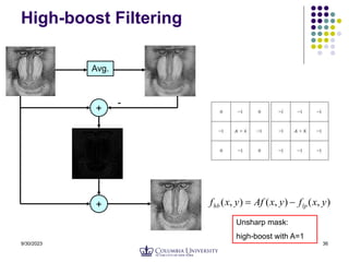
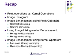
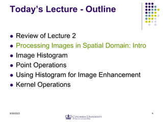
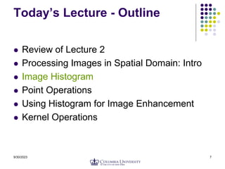
This document outlines a lecture on image enhancement in the spatial domain. It discusses processing images through point operations like thresholding, gamma correction, and contrast stretching. It also covers histogram modification techniques for image enhancement, including histogram equalization, specification, and adaptive equalization. Finally, it introduces kernel operations for spatial filtering, including smoothing, sharpening using derivatives, and high-boost filtering. The document provides examples and formulas for many of these common image enhancement techniques.

1. 9/30/2023 1
Lecture 3 (2.5.07)
Image Enhancement in
Spatial Domain
Shahram Ebadollahi
DIP ELEN E4830

2. 9/30/2023 2
Today’s Lecture - Outline
 Review of Lecture 2
 Processing Images in Spatial Domain: Intro
 Image Histogram
 Point Operations
 Using Histogram for Image Enhancement
 Kernel Operations

3. 9/30/2023 3
Today’s Lecture - Outline
 Review of Lecture 2
 Processing Images in Spatial Domain: Intro
 Image Histogram
 Point Operations
 Using Histogram for Image Enhancement
 Kernel Operations

4. 9/30/2023 4
Today’s Lecture - Outline
 Review of Lecture 2
 Processing Images in Spatial Domain: Intro
 Image Histogram
 Point Operations
 Using Histogram for Image Enhancement
 Kernel Operations

5. 9/30/2023 5
Processing Images in Spatial Domain:
Introduction
)
(
(.)
f
T
g
f N
T



 

N
y
M
x
y
x
f 


 1
,
1
,
)
,
( N
y
M
x
y
x
g 


 1
,
1
,
)
,
(
(.)
N
T : Spatial operator defined on a neighborhood N of a given pixel
)
,
(
0 y
x
N )
,
(
4 y
x
N )
,
(
8 y
x
N
point processing mask processing

6. 9/30/2023 6
Mask (filter, kernel, window, template)
processing
x
y
(0,0)
x
y
(0,0)
)
,
( y
x
f )
,
( y
x
g

7. 9/30/2023 7
Today’s Lecture - Outline
 Review of Lecture 2
 Processing Images in Spatial Domain: Intro
 Image Histogram
 Point Operations
 Using Histogram for Image Enhancement
 Kernel Operations

8. 9/30/2023 8
Image Histogram
 
MxN
r
n
m
f
MxN
n
k
h
L
h
k
h
h
h
H
r
r
r
r
n
m
f
f
m n
k
k
L
k
MxN
 




 
)
)
,
(
(
)
(
,
))
1
(
,
),
(
,
),
1
(
),
0
(
(
,
,
,
,
,
)
,
(
, 1
1
0





histogram
histogram
bi-level image
Pixel values linearly
increasing from 0 to
255 with increasing
column index
normalized
256x256
256x256
r
H
r
H
255
255
0
0.5
0
1/256

9. 9/30/2023 9
Image Histogram: example

10. 9/30/2023 10
Today’s Lecture - Outline
 Review of Lecture 2
 Processing Images in Spatial Domain: Intro
 Image Histogram
 Point Operations
 Using Histogram for Image Enhancement
 Kernel Operations

11. 9/30/2023 11
Point Processing:
Thresholding
))
,
(
(
)
,
(
)
,
( y
x
f
T
y
x
g
y
x
f 


)
(

 T



Input gray-level value Output gray-level value

)
(
 T

0

2


12. 9/30/2023 12
Point Processing:
Gamma Correction

cr
s 

13. 9/30/2023 13
Point Processing:
Contrast Stretching

















1
,
)
(
,
)
(
0
,
2
2
2
3
2
1
1
1
2
1
1
L
s
s
s















f g
f
H g
H

)
(
 T

2

1

2

1

0 L-1
1
s
2
s
3
s
L-1

14. 9/30/2023 14
Point Processing:
Clipping & Thresholding
f

)
(
 T

2

1

0 L-1
s

)
(
 T

1

0 L-1
clipping
thresholding
clip
g
thresh
g

15. 9/30/2023 15
Point Processing:
Gray-level Slicing

)
(
 T

2

1

0 L-1

)
(
 T

2

1

0 L-1

16. 9/30/2023 16
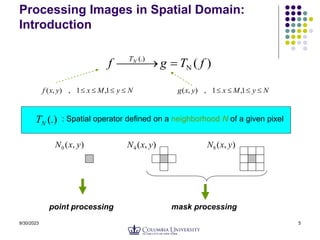
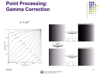
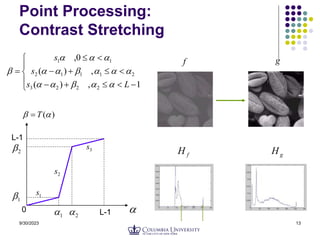
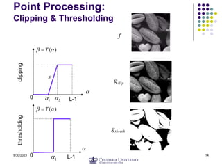
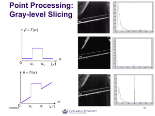
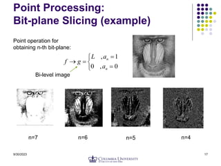
Point Processing:
Bit-plane Slicing
0
1
2
2
1
1 2
2
2
2 a
a
a
a
a
f n
B
n
B
B
B
B
B 





 




 

]
[ 0
1
2
1 a
a
a
a
a n
B
B
B 
 


10011101
157 

f
e.g.
1
2 

 n
n
n i
i
a






 n
n
f
i
2
where,
lsb
msb

17. 9/30/2023 17
Point Processing:
Bit-plane Slicing (example)







0
,
0
1
,
n
n
a
a
L
g
f
Point operation for
obtaining n-th bit-plane:
n=7 n=6 n=5 n=4
Bi-level image

18. 9/30/2023 18
Today’s Lecture - Outline
 Review of Lecture 2
 Processing Images in Spatial Domain: Intro
 Image Histogram
 Point Operations
 Using Histogram for Image Enhancement
 Kernel Operations

19. 9/30/2023 19
Histogram Modification
 Apply a transform to an image such that the resulting
image has desired histogram.
 Histogram Equalization (linearization)
 Histogram Specification (matching)
 Non-adaptive vs. Adaptive Histogram Modification
 Global histogram
 Local histogram

20. 9/30/2023 20
Histogram Equalization
Source
image
Equalized
Image
Corresponding
Histograms

21. 9/30/2023 21
Histogram Equalization
 Often images poorly use the full range of the
gray scale
 Solution:
Transform image such that its histogram is spread
out more evenly in gray scale
 Rather than guessing the parameters and the
form of the transformation use original gray-
scale distribution as the cue

22. 9/30/2023 22
Histogram Equalization
Histogram
Equalization
r s
r
p
s
p
(.)
T
ds
dr
r
p
s
p r
s )
(
)
( 



r
r du
u
p
r
T
s
0
)
(
)
(
1
)
( 
s
ps

 




k
j
j
k
j
j
r
k
k
MxN
n
r
p
r
T
s
0
0
)
(
)
(
# pixels with the
j-th gray-level
image size
Point operation for
equalizing histogram
for the example image
(.)
T

23. 9/30/2023 23
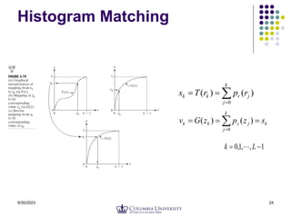
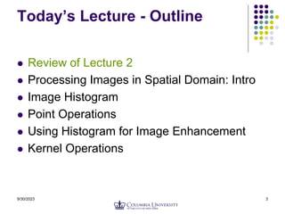
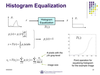
Histogram Matching
 Transform image such that resulting image has
specified histogram



r
r du
u
p
r
T
s
0
)
(
)
(
Histogram
Matching
r z
r
p (.)
F z
p
 

z
z s
dt
t
p
z
G
0
)
(
)
(
)]
(
[
)
( 1
1
r
T
G
s
G
z 


 T
G
F 1



24. 9/30/2023 24
Histogram Matching




k
j
j
r
k
k r
p
r
T
s
0
)
(
)
(
k
k
j
j
z
k
k s
z
p
z
G
v 

 
0
)
(
)
(
1
,
,
1
,
0 
 L
k 

25. 9/30/2023 25
Adaptive Histogram Equalization
Note: local
structure revealed
x
y
(0,0)
)
,
( y
x
f
)
,
( y
x
H
Histogram
Equalization

26. 9/30/2023 26
Today’s Lecture - Outline
 Review of Lecture 2
 Processing Images in Spatial Domain: Intro
 Image Histogram
 Point Operations
 Using Histogram for Image Enhancement
 Kernel Operations

27. 9/30/2023 27
Kernel Operator: Intro
Note: need to handle
borders of the image

28. 9/30/2023 28
Kernel Operator: Intro
Spatial
Filtering
f g
(.)
(.) w
TN 
)
1
,
1
(
)
1
,
1
(
)
,
(
)
0
,
0
(
)
,
1
(
)
0
,
1
(
)
1
,
1
(
)
1
,
1
(
)
,
( 












 n
m
f
w
n
m
f
w
n
m
f
w
n
m
f
w
n
m
g 

 

 




a
a
i
b
b
j
j
n
i
m
f
j
i
w
n
m
g )
,
(
)
,
(
)
,
(
1
2 
a
1
2 
b
N
n
M
m




1
1 kernel

29. 9/30/2023 29
FT
FT
Low-pass filter
Smoothing: Image Averaging
* Image edges
are softened

30. 9/30/2023 30
Smoothing: Averaging (example)
3x3
5x5
15x15
9x9
35x35
original
Noise effect is gone,
but image edges are
heavily blurred also

31. 9/30/2023 31
Order Statistics Filter
)}
,
(
{
)
,
(
)
,
(
)
,
(
t
s
f
median
y
x
g
y
x
W
t
s 

)}
,
(
{
max
)
,
(
)
,
(
)
,
(
t
s
f
y
x
g
y
x
W
t
s 

)}
,
(
{
min
)
,
(
)
,
(
)
,
(
t
s
f
y
x
g
y
x
W
t
s 

original

32. 9/30/2023 32
Image Derivative

33. 9/30/2023 33
Image Sharpening: 1-st derivative

























y
f
x
f
G
G
f
y
x
Image gradient: y
x G
G
f 


Robert’s
operator
Sobel’s
operator
Sobel filter in
frequency
domain

34. 9/30/2023 34
Image Sharpening: 2-nd derivative
2
2
2
2
2
y
f
x
f
f







Image Laplacian:
)
,
(
2
)
,
1
(
)
,
1
(
2
2
y
x
f
y
x
f
y
x
f
x
f







)
,
(
2
)
1
,
(
)
1
,
(
2
2
y
x
f
y
x
f
y
x
f
y
f







)
,
(
4
)
1
,
(
)
1
,
(
)
,
1
(
)
,
1
(
2
y
x
f
y
x
f
y
x
f
y
x
f
y
x
f
f











35. 9/30/2023 35
Image Sharpening: 2-nd derivative
* +
Laplacian filter in
frequency
domain

36. 9/30/2023 36
High-boost Filtering
Avg.
+
+
-
)
,
(
)
,
(
)
,
( y
x
f
y
x
Af
y
x
f lp
hb 

Unsharp mask:
high-boost with A=1

37. 9/30/2023 37
Recap
 Point operations vs. Kernel Operations
 Image Histogram
 Image Enhancement using Point Operators
 Contrast Stretching
 Gamma Correction
 Using Image Histogram for Enhancement
 Histogram Equalization
 Histogram Matching
 Image Enhancement using Kernel Operators
 Low-pass filtering (averaging)
 High-pass filtering (sharpening)