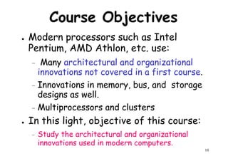
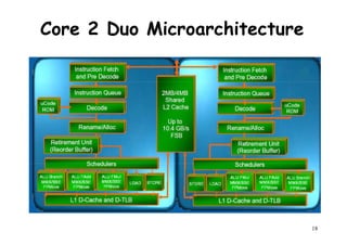
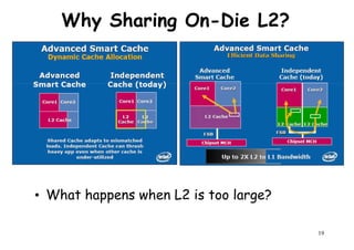
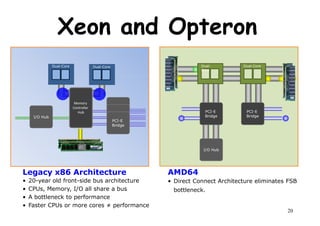
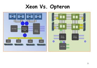
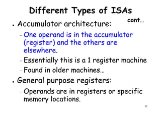
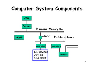
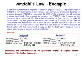
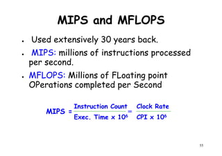
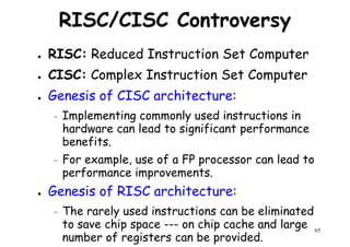
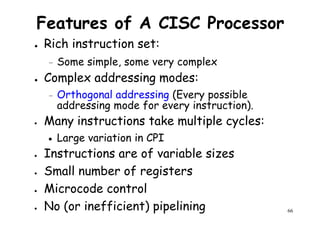
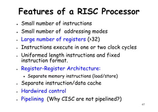
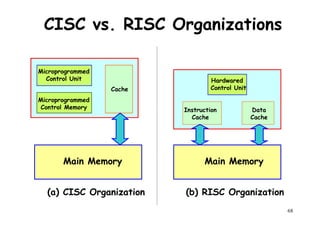
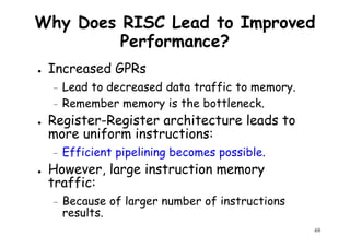
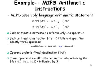
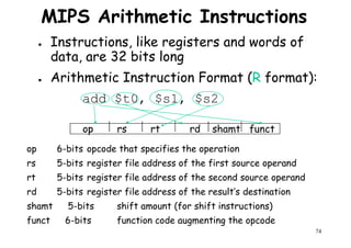
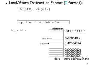
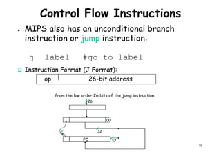
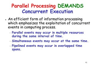
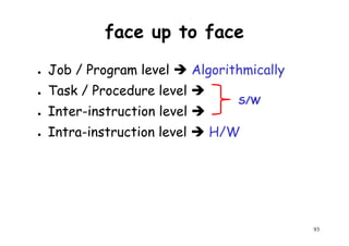
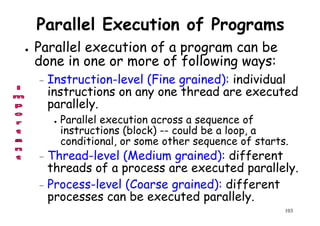
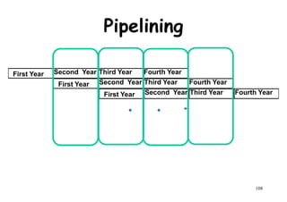
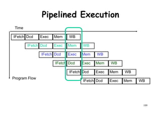
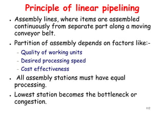
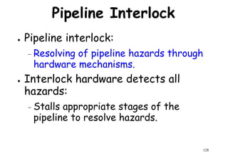
The document provides an introduction to computer architecture and performance. It discusses how performance has increased due to Moore's Law and transistor density doubling every 18 months. It explains that improvements in recent decades have come more from architectural innovations like pipelining than just manufacturing advances. Pipelining allows multiple instructions to be processed simultaneously to improve performance. The document outlines some objectives of studying innovations like RISC architectures, pipelining, caching and parallel processing.

1. High Performance
Computer Architecture
Introduction to Pipeline
1
Mr. SUBHASIS DASH
SCHOOL OF COMPUTER ENGINEERING.
KIIT UNIVERSITY
BHUBANESWAR

2. Introduction
– Computer performance has been
increasing phenomenally over theincreasing phenomenally over the
last five decades.
– Brought out by Moore’s Law:
● Transistors per square inch roughly double
every eighteen months.
Moore’s law is not exactly a law:
2
– Moore’s law is not exactly a law:
● but has held good for nearly 50 years.

3. Moore’s Law
Gordon Moore (co-founder of Intel)
3
Moore’s Law: it’s worked for
a long time
Gordon Moore (co-founder of Intel)
predicted in 1965: “Transistor density
of minimum cost semiconductor chips
would double roughly every 18
months.”
Transistor density is correlated to
processing speed.

4. Trends Related to Moore’s Law
Cont…
• Processor performance:
•Twice as fast after every 2 years
(roughly).
• Memory capacity:
•Twice as much after every 18 months
(roughly).
4
(roughly).

5. Interpreting Moore’s Law
● Moore's law is not about just the density of
transistors on a chip that can be achieved:
But about the density of transistors at which the– But about the density of transistors at which the
cost per transistor is the lowest.
● As more transistors are made on a chip:
– The cost to make each transistor reduces.
– But the chance that the chip will not work due to a
defect rises.
5
defect rises.
● Moore observed in 1965 there is a transistor
density or complexity:
– At which "a minimum cost" is achieved.

6. How Did Performance Improve?
● Till 1980s, most of the performance improvements
came from using innovations in manufacturing
technologies:technologies:
– VLSI
– Reduction in feature size
● Improvements due to innovations in manufacturing
technologies have slowed down since 1980s:
Smaller feature size gives rise to increased resistance,
6
– Smaller feature size gives rise to increased resistance,
capacitance, propagation delays.
– Larger power dissipation.
(Aside: What is the power consumption of Intel Pentium Processor?
Roughly 100 watts idle)

7. How Did Performance Improve?
Cont…
● Since 1980s, most of the
performance improvements haveperformance improvements have
come from:
– Architectural and organizational
innovations
What is the difference between:
7
● What is the difference between:
– Computer architecture and computer
organization?

8. Architecture vs. Organization
● Architecture:
– Also known as Instruction Set Architecture– Also known as Instruction Set Architecture
(ISA)
– Programmer visible part of a processor:
instruction set, registers, addressing modes, etc.
● Organization:
– High-level design: how many caches? how many
8
– High-level design: how many caches? how many
arithmetic and logic units? What type of
pipelining, control design, etc.
– Sometimes known as micro-architecture

9. Computer Architecture
● The structure of a computer that a
machine language programmer mustmachine language programmer must
understand:
– To be able to write a correct program for
that machine.
● A family of computers of the same
architecture should be able to run the
9
architecture should be able to run the
same program.
– Thus, the notion of architecture leads to
“binary compatibility.”

10. Course Objectives
● Modern processors such as Intel
Pentium, AMD Athlon, etc. use:Pentium, AMD Athlon, etc. use:
– Many architectural and organizational
innovations not covered in a first course.
– Innovations in memory, bus, and storage
designs as well.
– Multiprocessors and clusters
10
– Multiprocessors and clusters
● In this light, objective of this course:
– Study the architectural and organizational
innovations used in modern computers.

11. A Few Architectural and
Organizational Innovations
Course Objectives
RISC (Reduced Instruction Set● RISC (Reduced Instruction Set
Computers):
– Exploited instruction-level parallelism:
● Initially through pipelining and later by using
multiple instruction issue (superscalar)
11
multiple instruction issue (superscalar)
– Use of on-chip caches
● Dynamic instruction scheduling
● Branch prediction

12. Intel MultiCore Architecture
● Improving execution rate of a single-
thread is still considered important:
Uses out-of-order execution and speculation.– Uses out-of-order execution and speculation.
● MultiCore architecture:
– Can reduce power consumption.
– (14 pipeline stages) is closer to the Pentium
M (12 stages) than the P4 (30 stages).
12
M (12 stages) than the P4 (30 stages).
● Many transistors are invested in large
branch predictors:
– To reduce wasted work (power).

13. Intel’s Dual Core Architectures
● The Pentium D is simply two Pentium 4 cpus:
– Inefficiently paired together to run as dual core.
● Core Duo is Intel's first generation dual core processor● Core Duo is Intel's first generation dual core processor
based upon the Pentium M (a Pentium III-4 hybrid):
– Made mostly for laptops and is much more efficient than
Pentium D.
● Core 2 Duo is Intel's second generation (hence, Core
2) processor:
13
– Made for desktops and laptops designed to be fast while
not consuming nearly as much power as previous CPUs.
● Intel has now dropped the Pentium name in favor of
the Core architecture.

14. Intel Core Processor
14

15. Intel Core 2 Duo
• Code named “conroe”
• Homogeneous cores• Homogeneous cores
• Bus based chip
interconnect.
• Shared on-die Cache
Memory.
15
Memory.
Classic OOO: Reservation
Stations, Issue ports,
Schedulers…etc Large, shared set
associative, prefetch, etc.
Source: Intel Corp.

16. Intel’s Core 2 Duo
● Launched in July 2006.
– Replacement for Pentium 4 and Pentium D CPUs.
Intel claims:● Intel claims:
– Conroe provides 40% more performance at
40% less power compared to the Pentium D.
● All Conroe processors are manufactured
with 4 MB L2 cache:
Due to manufacturing defects, the E6300 and
16
– Due to manufacturing defects, the E6300 and
E6400 versions based on this core have half
their cache disabled, leaving them with only
2 MB of usable L2 cache.

17. Intel Core Processor
Specification
● Speeds:1.06 GHz to 3 GHz
FSB speeds:533 MT/s to 1333 MT/s● FSB speeds:533 MT/s to 1333 MT/s
● Process: 0.065 µm (MOSFET channel
length)
● Instruction set:x86, MMX, SSE, SSE2,
SSE3, SSSE3, x86-64
17
SSE3, SSSE3, x86-64
● Microarchitecture: Intel Core
microarchitecture
● Cores:1, 2, or 4 (2x2)

18. Core 2 Duo Microarchitecture
18

19. Why Sharing On-Die L2?
19
• What happens when L2 is too large?

20. Xeon and Opteron
Dual-Core Dual-Core Dual-CoreDual-
Core
I/O Hub
PCI-E
BridgeI/O Hub
PCI-E
Bridge
PCI-E
Bridge
PCI-E
Bridge
Memory
Controller
Hub PCI-E
Bridge
20
I/O Hub
Legacy x86 Architecture
• 20-year old front-side bus architecture
• CPUs, Memory, I/O all share a bus
• A bottleneck to performance
• Faster CPUs or more cores ≠ performance
AMD64
• Direct Connect Architecture eliminates FSB
bottleneck.

21. Dual-Core Dual-Core Dual-CoreDual-Core
Dual-
Core
Dual-
Core
Xeon Vs. Opteron
PCI-E
Bridge
PCI-E
Bridge
PCI-E
Bridge
PCI-E
Bridge
PCI-E
Bridge
I/O Hub
XMBXMB XMB XMB
Memory
Controller
Hub
Dual-
Core
Dual-
Core
21
21
I/O Hub

22. Now as for why, let me also try to explain that.
There are numerous reasons, the FSB is one, but not the only one.
The biggest factor is something called instructions per clock cycle (IPC).
WHY
The biggest factor is something called instructions per clock cycle (IPC).
The Ghz number of a processor shows how fast the clock cycles are.
But the Core 2 Duo has a much higher IPC, meaning it processes more data
each clock cycle than the Pentium D.
Put into its simplest terms, think of it this way, say the Pentium D has 10
clock cycles in a given amount of time, while the Core 2 Duo would have only 6.
But the Core 2 Duo could processor 10 instruction per clock cycle, but the
22
But the Core 2 Duo could processor 10 instruction per clock cycle, but the
Pentium D only 4.
In the given amount of time, the Core 2 Duo would process 60 instructions,
but the Pentium D only 40.
This is why it actually performs faster even with a lower clock speed.

23. Today’s Objectives
● Study some preliminary concepts:
Amdahl’s law, performance– Amdahl’s law, performance
benchmarking, etc.
● RISC versus CISC architectures.
● Types of parallelism in programs
versus types of parallel
23
versus types of parallel
computers.
● Basic concepts in pipelining.

24. Measuring performance
● Real Application
– Problems occurs due to the dependencies on– Problems occurs due to the dependencies on
OS or COMPILER
● Modified Application
– To enhance the probability of need
– Focus on one particular aspect of the system
performance
24
performance
● Kernels
– To isolate performance of individual features
of M/c

25. Toy Benchmarks
● The performance of different
computers can be compared by running
some standard programs:
computers can be compared by running
some standard programs:
– Quick sort, Merge sort, etc.
● But, the basic problem remains:
– Even if you select based on a toy
benchmark, the system may not perform
25
Even if you select based on a toy
benchmark, the system may not perform
well in a specific application.
– What can be a solution then?

26. Synthetic Benchmarks
● Basic Principle: Analyze the distribution of
instructions over a large number of practical
programs.programs.
● Synthesize a program that has the same
instruction distribution as a typical program:
– Need not compute something meaningful.
● Dhrystone, Khornerstone, Linpack are some
of the older synthetic benchmarks:
26
● Dhrystone, Khornerstone, Linpack are some
of the older synthetic benchmarks:
– More recent is SPEC..( Standard performance
evaluation corporation )

27. SPEC Benchmarks
● SPEC: Standard Performance Evaluation
Corporation:
– A non-profit organization (www.spec.org)
● CPU-intensive benchmark for evaluating
processor performance of workstation:
– Generations: SPEC89, SPEC92, SPEC95,
and SPEC2000 …
27
and SPEC2000 …
– Emphasizing memory system performance
in SPEC2000.

28. Problems with Benchmarks
● SPEC89 benchmark included a small
kernel called matrix 300:kernel called matrix 300:
– Consists of 8 different 300*300 matrix
operations.
– Optimization of this inner-loop resulted in
performance improvement by a factor of 9.
Optimizing performance can discard 25%
28
● Optimizing performance can discard 25%
Dhrystone code
● Solution: Benchmark suite

29. Other SPEC Benchmarks
● SPECviewperf: 3D graphics performance
– For applications such as CAD/CAM, visualization,– For applications such as CAD/CAM, visualization,
content creations, etc.
● SPEC JVM98: performance of client-side
Java virtual machine.
● SPEC JBB2000: Server-side Java application
SPEC WEB2005: evaluating WWW servers
29
● SPEC WEB2005: evaluating WWW servers
– Contains multiple workloads utilizing both http
and https, dynamic content implemented in PHP
and JSP.

30. BAPCo
● Non-profit consortium
www.bapco.comwww.bapco.com
● SYSmark 2004 SE
– Office productivity benchmark
30

31. Instruction Set Architecture
(ISA)
● Programmer visible part of a processor:
– Instruction Set (what operations can be– Instruction Set (what operations can be
performed?)
– Instruction Format (how are instructions
specified?)
– Registers (where are data located?)
31
– Addressing Modes (how is data accessed?)
– Exceptional Conditions (what happens if
something goes wrong?)

32. ISA cont…
● ISA is important:
– Not only from the programmer’s
perspective.
– From processor design and
implementation perspectives as well.
32

33. Evolution of Instruction Sets
Single Accumulator
(Manchester Mark I,(Manchester Mark I,
IBM 700 series 1953)
General Purpose Register Machines
Complex Instruction Sets RISC
(Vax, Intel 386 1977-85)
(MIPS,IBM RS6000, . . .1987)
Stack
(Burroughs, HP-3000 1960-70)
33
(Vax, Intel 386 1977-85)
(MIPS,IBM RS6000, . . .1987)

34. Different Types of ISAs
● Determined by the means used for
storing data in CPU:storing data in CPU:
● The major choices are:
– A stack, an accumulator, or a set of
registers.
Stack architecture:
34
● Stack architecture:
– Operands are implicitly on top of the
stack.

35. Different Types of ISAs
cont…
● Accumulator architecture:
– One operand is in the accumulator
(register) and the others are
– One operand is in the accumulator
(register) and the others are
elsewhere.
– Essentially this is a 1 register machine
– Found in older machines…
General purpose registers:
35
● General purpose registers:
– Operands are in registers or specific
memory locations.

36. Comparison of Architectures
Consider the operation: C =A + BConsider the operation: C =A + B
Stack Accumulator Register-Memory Register-Register
Push A Load A Load R1, A Load R1, A
Push B Add B Add R1, B Load R2, B
Add Store C Store C, R1 Add R3, R1, R2
36
Add Store C Store C, R1 Add R3, R1, R2
Pop C Store C, R3

37. Types of GPR Computers
● Register-Register (0,3)Register-Register (0,3)
● Register-Memory (1,2)
● Register-Memory (2,2) (3,3)
37

38. Quantitative Principle of
Computer Design
● MAKE COMMON CASE FAST
Frequent case over infrequent case– Frequent case over infrequent case
– Improvement is easy to the Frequent case
– Quantifies overall performance gain due to
improve in the part of computation.
38

39. Computer System Components
CPU
Caches
RAM
Adapter
Peripheral Buses
Processor-Memory Bus
39
Controllers Controllers
I/O devices
Displays
Keyboards
Networks

40. Amdahl’s Law
● Quantifies overall performance gain due to
improve in a part of a computation. (CPU Bound)
Amdahl’s Law:● Amdahl’s Law:
– Performance improvement gained from using some
faster mode of execution is limited by the amount
of time the enhancement is actually used
Performance for entire task using enhancement when possible
Speedup =
40
Performance for entire task without using enhancement
Speedup =
Execution time for the task using enhancement
Execution time for a task without enhancement
Speedup =
OR

41. Amdahl’s Law and Speedup
● Speedup tells us:
– How much faster a machine will run due to an
enhancement.enhancement.
● For using Amdahl’s law two things should
be considered:
– 1st… FRACTION ENHANCED :-Fraction of the
computation time in the original machine
41
computation time in the original machine
that can use the enhancement
– It is always less than or equal to 1
● If a program executes in 30 seconds and 15
seconds of exec. uses enhancement, fraction = ½

42. Amdahl’s Law and Speedup
– 2nd… SPEEDUP ENHANCED :-Improvement
gained by enhancement, that is how
much faster the task would run if themuch faster the task would run if the
enhanced mode is used for entire
program.
– Means the time of original mode over
the time of enhanced mode
It is always greater than 1
42
– It is always greater than 1
● If enhanced task takes 3.5 seconds and
original task took 7secs, we say the
speedup is 2.

43. Amdahl’s Law Equations
Execution timenew = Execution timeold x (1 – Fractionenhanced) +
Fractionenhanced
SpeedupSpeedupenhanced
Speedupoverall =
Execution Timeold
Execution Timenew
=
(1 – Fractionenhanced) +
Fractionenhanced
Speedupenhanced
1
Use previous equation,
Solve for speedup
43
Don’t just try to memorize
these equations and plug numbers into them.
It’s always important to think about the problem too!

44. Amdahl’s Law Example
● Suppose that we are considering an enhancement to
the processor of a server system used for web
serving. The new CPU is 10 times faster on
computation in the web serving application than thecomputation in the web serving application than the
original processor. Assuming that the original CPU is
busy with computation 40% of the time & is waiting
for I/O 60% of the time. What is the overall speed
up gained by incorporating the enhancement?
● Solution:- Fractionenhanced = 0.4
Speedup = 10
44
Speedupenhanced = 10
Speedupoverall = = 1.56
1
(1 – 0.4) + (0.4/10)
~

45. Corollary of Amdahl’s Law
1. Amdahl’s law express the law of diminishing
returns. The incremental improvement in speed
up gained by an additional improvement in theup gained by an additional improvement in the
performance of just a portion of the
computation diminishes as improvements are
added.
1. If an enhancement is only usable for a fraction
45
1. If an enhancement is only usable for a fraction
of task, we can’t speed up the task by more
than the reciprocal of (1- Fraction Enhanced ).

46. Amdahl’s Law Example
Assume that we make an enhancement to a computer that improves some mode
of execution by a factor of 10. Enhanced mode is used 50% of the time.
Measured as a percentage of the execution time when the enhanced mode is in
use. Recall that Amdahl’s law depends on the fraction of the original,
Unenhanced execution time that could make use of enhanced mode. Thus we
can’t directly use this 50% measurement to compute speed up with Amdahl’s
law. What is the speed up we have obtained from the fast mode? What
● Solution:- If an enhancement is only usable for a fraction of task, we can’t
speed up the task by more than the reciprocal of (1- Fraction).
● Speedup = = 1/(1-0.5) = 2
(1 – Fractionenhanced)
1
law. What is the speed up we have obtained from the fast mode? What
percentage of the original execution time has been converted to fast mode?
46
●
Speedupoverall =
1
(1 – Fractionenhanced) +
Fractionenhanced
Speedupenhanced
(1 – Fractionenhanced) +
Fractionenhanced
10
1
2 =

47. Amdahl’s Law -Example
● A common transformation required in graphics engines is SQRT. Implementations of
FPSQRT is vary significantly in performance, especially among processors designed for
graphics. Suppose FPSQRT is responsible for 20% of the execution time of a critical
graphics benchmark. One proposal to enhance the FPSQRT H/W & speed up this
operation by a factor of 10. The other alternative is just to try to make FP
instructions in the graphics processor run faster by a factor of 1.6. The FPinstructions in the graphics processor run faster by a factor of 1.6. The FP
instructions are responsible for a total of 50% of the execution time for the
application. The design team believes that they can make all FP instructions run 1.6
times faster with the same effort as required for the fast SQRT. Compare these 2
design alternatives to suggest which one is better.
● Solution:-
Design 1
Fraction Enhanced= 20% 0.2
Design 2
Fraction Enhanced= 50% 0.5
Speed up = 1.6
47
Fraction Enhanced= 20% 0.2
Speed up Enhanced = 10
Seed up FPSQRT Overall = 1/ (1-0.2) + (0.2/10)
= 1/0.82 ~ 1.22
Fraction Enhanced= 50% 0.5
Speed up Enhanced = 1.6
Seed up FP Overall = 1/ (1-0.5) + (0.5/1.6)
= 1/0.8125 ~ 1.23
Improving the performance of FP operations overall is slightly better
because of the higher frequency .
= =

48. Advanced Computer
Architectures
Lecture-2:Lecture-2:
A Few Basic Concepts
48
Mr. SUBHASIS DASH
SCHOLE OF COMPUTER SCIENCE & ENGG.
KIIT UNIVERSITY
BHUBANESWAR

49. CPU Performance Equation
● Computers using a clock running at a constant
rate.
CPU time = CPU clock cycles for a program X● CPU time = CPU clock cycles for a program X
clock cycle time
CPU clock cycles for a program
Clock Rate
=
CPI can be defined in terms of No. of clock cycles & instruction
49
CPI can be defined in terms of No. of clock cycles & instruction
count. ( IPC CPI)
CPU clock cycles for a program
Instruction count
CPI =

50. CPU Performance Equation
● CPU time = Instruction count X clock cycle
time X cycle per instruction.
● CPU time = × ×
● Performance dependant on 3 parameter
Clock Cycle Time ( H/W technology & Organization)
Instruction
Program Instruction
Clock cycle
Clock cycle
Second
50
– Clock Cycle Time ( H/W technology & Organization)
– CPI ( Organization & ISA )
– IC ( ISA & Compiler Technology )

51. CPU Performance Equation
● CPU clock cycle = Σ
i=1
n
IC i X CPI i Where :-
IC No. of times
● CPI overall
=
i=1
IC i X CPI iΣ
i=1
n
Instruction Count
IC I No. of times
instructions i
is executed in
a program.
CPI I Average No.
of clock pre
instructions.
51
instructions.

52. Performance Measurements
● Performance measurement is
important:important:
– Helps us to determine if one
processor (or computer) works
faster than another.
A computer exhibits higher
52
– A computer exhibits higher
performance if it executes programs
faster.

53. Clock-Rate Based Performance
Measurement
● Comparing performance based on
clock rates is obviously meaningless:clock rates is obviously meaningless:
– Execution time=CPI × Clock cycle time
– Please remember:
● Higher CPI need not mean better
performance.
53
performance.
● Also, a processor with a higher clock
rate may execute programs much
slower!

54. Example: Calculating Overall
CPI (Cycles per Instruction)
Operation Freq CPI(i) (% Time)
ALU 50% 1 (40%)
Typical Instruction Mix
ALU 50% 1 (40%)
Load 20% 2 (27%)
Store 10% 2 (13%)
Branch 20% 5 (20%)
54
Overall CPI= 1*0.4+ 2*0.27+ 2*0.13+5*0.2
= 2.2

55. MIPS and MFLOPS
● Used extensively 30 years back.
MIPS: millions of instructions processed● MIPS: millions of instructions processed
per second.
● MFLOPS: Millions of FLoating point
OPerations completed per Second
Instruction Count Clock Rate
55
MIPS =
Exec. Time x 106
Instruction Count
CPI x 106
Clock Rate
=

56. Problems with MIPS
● Three significant problems with
using MIPS:using MIPS:
● So severe, made some one term:
– “Meaningless Information about
Processing Speed”
Problem 1:
56
● Problem 1:
– MIPS is instruction set dependent.

57. Problems with MIPS
cont…
● Problem 2:
MIPS varies between programs on– MIPS varies between programs on
the same computer.
● Problem 3:
– MIPS can vary inversely to
performance!
57
performance!
● Let’s look at an example as to why
MIPS doesn’t work…

58. A MIPS Example
● Consider the following computer:
Code type- A B C
Instruction counts (in millions) for each
instruction class
Code type- A (1 cycle) B (2 cycle) C (3 cycle)
Compiler 1 5 1 1
Compiler 2 10 1 1
instruction class
The machine runs at 100MHz.
Instruction A requires 1 clock cycle, Instruction B requires 2
clock cycles, Instruction C requires 3 clock cycles.
58
clock cycles, Instruction C requires 3 clock cycles.
Σ CPIi x Ni
i =1
n
CPI =
Instruction Count
CPU Clock Cycles
Instruction Count
=

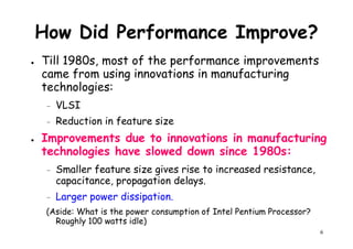
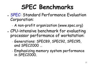
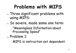
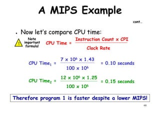
59. A MIPS Example
cont…
CPI1 =
(5 + 1 + 1) x 106
[(5x1) + (1x2) + (1x3)] x 106
10/7 = 1.43=
count cycles
(5 + 1 + 1) x 106
MIPS1 =
1.43
100 MHz
69.9=
CPI2 =
(10 + 1 + 1) x 106
[(10x1) + (1x2) + (1x3)] x 106
15/12 = 1.25=
59
(10 + 1 + 1) x 106
MIPS2 =
1.25
100 MHz
80.0=
So, compiler 2 has a higher
MIPS rating and should be
faster?

60. A MIPS Example
cont…
● Now let’s compare CPU time:
Instruction Count x CPINote
CPU Time =
Clock Rate
Instruction Count x CPI
= 0.10 secondsCPU Time1 =
100 x 106
7 x 106 x 1.43
12 x 106 x 1.25
!
Note
important
formula!
60
= 0.15 secondsCPU Time2 =
100 x 106
12 x 106 x 1.25
Therefore program 1 is faster despite a lower MIPS!Therefore program 1 is faster despite a lower MIPS!

61. CPU Performance Equation
● Suppose we have made the following measurements :-
Frequency of FP operations (Other than FPSQRT) = 25 %– Frequency of FP operations (Other than FPSQRT) = 25 %
– Average CPI of FP operations = 4.0
– Average CPI of other operations = 1.33
– Frequency of FPSQRT = 2%
– CPI of FPSQRT = 20
– Assume that the 2 design alternatives are to decrease the CPI of
61
– Assume that the 2 design alternatives are to decrease the CPI of
FPSQRT to 2 or to decrease the average CPI Of all FP operations to
2.5. Compare these 2 design alternatives using the CPU performance
equation.

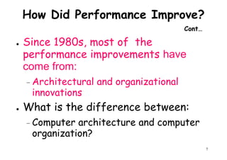
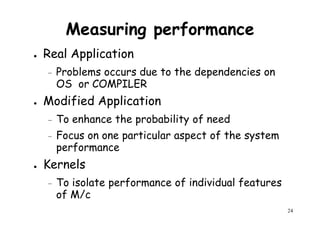
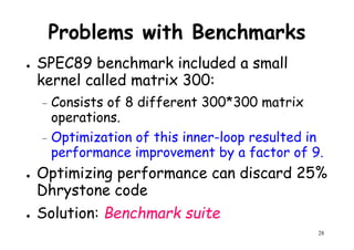
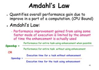
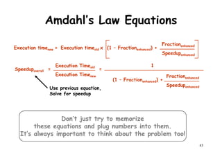
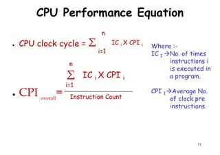
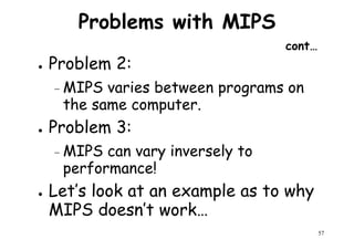
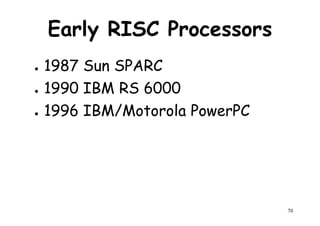
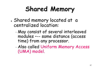
62. CPU Performance Equation
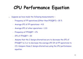
● Suppose we have made the following measurements :-
– Frequency of FP operations (Other than FPSQRT) = 25 %
– Average CPI of FP operations = 4.0
– Average CPI of other operations = 1.33Average CPI of other operations = 1.33
– Frequency of FPSQRT = 2%
– CPI of FPSQRT = 20
– Assume that the 2 design alternatives are to decrease the CPI of FPSQRT to 2 or
to decrease the average CPI Of all FP operations to 2.5. Compare these 2 design
alternatives using the CPU performance equation.
● Solutions:- First observe that only the CPI changes, the clock rate and instruction
count remain identical. We can start by finding original CPI without enhancement:-
n
62
We can compute the CPI for the enhanced FPSQRT by subtracting the cycles saved from
the original CPI :-
CPI with new FPSQRT = CPI Original – [2% x (CPI old FPSQRT – CPI new FPSQRT)]
= 2 – [(2/10)x (20-2)] = 1.64
Σ CPIi x Ni
i =1
n
Instruction Count
CPU Clock Cycles
Instruction Count
=CPI original = = (4 x 25%) + (1.33 x 75%) ~ 2
=

63. CPU Performance Equation
● We can compute the CPI for the enhanced of all FP instructions the same way or by
adding FP and NON FP CPIs.
● CPI new FP = (75% x 1.33) + (25% x 2.5) = 1.6225
● Since the CPI of the overall FP enhancement is slightly lower, its performance will be
marginally better, specifically the speed up for the overall FP enhancement is :-marginally better, specifically the speed up for the overall FP enhancement is :-
● Speed up over all for FP = 2/1.6225 = 1.23
● Speed up over all for FPSQRT = 2/1.64 = 1.22
63

64. Today’s Objectives
● Study some preliminary concepts:
Amdahl’s law, performance– Amdahl’s law, performance
benchmarking, etc.
● RISC versus CISC architectures.
● Types of parallelism in programs
versus types of parallel
64
versus types of parallel
computers.
● Basic concepts in pipelining.

65. RISC/CISC Controversy
● RISC: Reduced Instruction Set Computer
● CISC: Complex Instruction Set ComputerCISC: Complex Instruction Set Computer
● Genesis of CISC architecture:
– Implementing commonly used instructions in
hardware can lead to significant performance
benefits.
– For example, use of a FP processor can lead to
performance improvements.
65
– For example, use of a FP processor can lead to
performance improvements.
● Genesis of RISC architecture:
– The rarely used instructions can be eliminated
to save chip space --- on chip cache and large
number of registers can be provided.

66. Features of A CISC Processor
● Rich instruction set:
– Some simple, some very complex
Complex addressing modes:● Complex addressing modes:
– Orthogonal addressing (Every possible
addressing mode for every instruction).
• Many instructions take multiple cycles:
• Large variation in CPI
Instructions are of variable sizes
66
• Instructions are of variable sizes
• Small number of registers
• Microcode control
• No (or inefficient) pipelining

67. Features of a RISC Processor
● Small number of instructions
● Small number of addressing modes
Large number of registers (>32)• Large number of registers (>32)
• Instructions execute in one or two clock cycles
• Uniformed length instructions and fixed
instruction format.
• Register-Register Architecture:
• Separate memory instructions (load/store)
67
• Separate memory instructions (load/store)
• Separate instruction/data cache
• Hardwired control
• Pipelining (Why CISC are not pipelined?)

68. CISC vs. RISC Organizations
Microprogrammed
Control UnitControl Unit
Microprogrammed
Control Memory
Cache
Hardwared
Control Unit
Instruction
Cache
Data
Cache
68
Main Memory Main Memory
(a) CISC Organization (b) RISC Organization

69. Why Does RISC Lead to Improved
Performance?
● Increased GPRs
Lead to decreased data traffic to memory.– Lead to decreased data traffic to memory.
– Remember memory is the bottleneck.
● Register-Register architecture leads to
more uniform instructions:
– Efficient pipelining becomes possible.
However, large instruction memory
69
● However, large instruction memory
traffic:
– Because of larger number of instructions
results.

70. Early RISC Processors
● 1987 Sun SPARC
● 1990 IBM RS 6000
● 1996 IBM/Motorola PowerPC
70

71. ● Instruction Categories
– Computational
– Load/Store
R0 - R31
Registers
MIPS R3000 Instruction Set Architecture (ISA)
– Load/Store
– Jump and Branch
– Floating Point
● coprocessor
– Memory Management
– Special
PC
HI
LO
71
– Special
OP
OP
OP
rs rt rd sa funct
rs rt immediate
jump target
3 Instruction Formats: all 32 bits wide
R format
I format
J format

72. ● Holds thirty-two 32-bit
registers
– Two read ports and
One write port
Register File
src1 addr
src2 addr
dst addr
32 bits
src1
data32
locations
325
5
5
MIPS Register File
– One write port
Registers are
Faster than main memory
- But register files with more locations are slower
(e.g., a 64 word file could be as much as 50% slower
dst addr
write data
src2
data
locations
32
5
32
write
control
72
(e.g., a 64 word file could be as much as 50% slower
than a 32 word file)
- Read/write port affected by speed
Can hold variables so that
- code density improves (since register are named with
fewer bits than a memory location)

73. ● MIPS assembly language arithmetic statement
add $t0, $s1, $s2
Example:- MIPS Arithmetic
Instructions
sub $t0, $s1, $s2
Each arithmetic instruction performs only one operation
Each arithmetic instruction fits in 32 bits and specifies
exactly three operands
destination ← source1 op source2
73
destination ← source1 op source2
Operand order is fixed (destination first)
Those operands are all contained in the datapath’s register
file ($t0,$s1,$s2) – indicated by $

74. ● Instructions, like registers and words of
data, are 32 bits long
● Arithmetic Instruction Format (R format):
MIPS Arithmetic Instructions
● Arithmetic Instruction Format (R format):
add $t0, $s1, $s2
op rs rt rd shamt funct
op 6-bits opcode that specifies the operation
rs 5-bits register file address of the first source operand
74
rs 5-bits register file address of the first source operand
rt 5-bits register file address of the second source operand
rd 5-bits register file address of the result’s destination
shamt 5-bits shift amount (for shift instructions)
funct 6-bits function code augmenting the opcode

75. op rs rt 16 bit offset
● Load/Store Instruction Format (I format):
lw $t0, 24($s2)
op rs rt 16 bit offset
Memory
0xf f f f f f f f
$s2 0x12004094
2410 + $s2 =
0x120040ac$t0
75
data word address (hex)
0x00000000
0x00000004
0x00000008
0x0000000c

76. ● MIPS also has an unconditional branch
instruction or jump instruction:
Control Flow Instructions
j label #go to label
Instruction Format (J Format):
op 26-bit address
26
from the low order 26 bits of the jump instruction
76
PC
4
32
32
00

77. MIPS Control Flow Instructions
● MIPS conditional branch instructions:
bne $s0, $s1, Lbl #go to Lbl if $s0≠$s1
beq $s0, $s1, Lbl #go to Lbl if $s0=$s1beq $s0, $s1, Lbl #go to Lbl if $s0=$s1
– Ex: if (i==j) h = i + j;
bne $s0, $s1, Lbl1
add $s3, $s0, $s1
Lbl1: ...
77
How is the branch destination address specified?

78. Specifying Branch Destinations
● Use a register (like in load) added to the 16-
bit offset
– which register? Instruction Address Register
(the PC)(the PC)
● its use is automatically implied by instruction
● PC gets updated (PC+4) during the fetch cycle so that it holds the address
of the next instruction
offset
16
sign-extend
from the low order 16 bits of the branch instruction
78
PC
Add
32
32
32
32
32
32
00
sign-extend
branch dst
address
?
Add
4
32

79. 79

80. 80

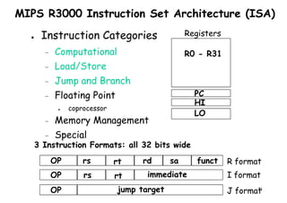
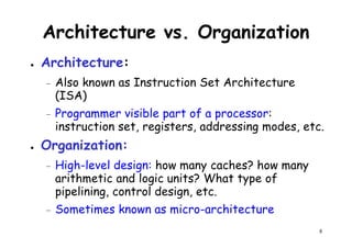
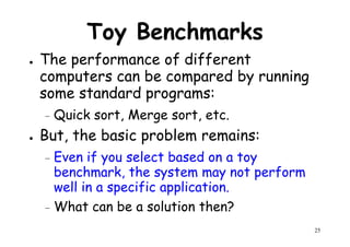
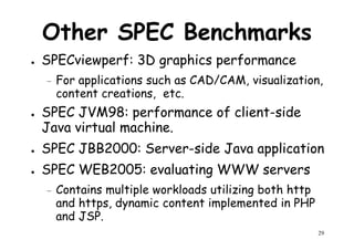
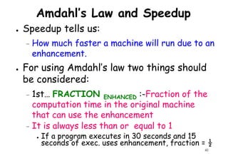
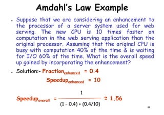
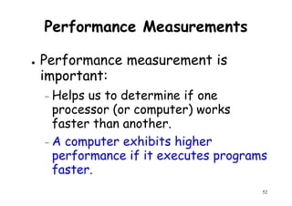
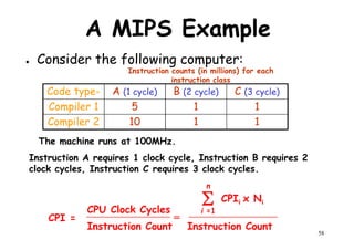
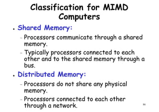
81. Architectural Classifications
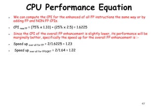
● Flynn’s Classifications [1966]
Based on multiplicity of instruction streams– Based on multiplicity of instruction streams
& data stream in a computer.
● Feng’s Classification [1972]
– Based on serial & parallel processing.
● Handler’s Classification [1977]
81
Handler’s Classification [1977]
– Determined by the degree of parallelism &
pipeline in various subsystem level.

82. Flynn’s Classification
● SISD (Single Instruction Single Data):
– Uniprocessors.
MISD (Multiple Instruction Single● MISD (Multiple Instruction Single
Data):
– No practical examples exist
● SIMD (Single Instruction Multiple
Data):
– Specialized processors
82
– Specialized processors
● MIMD (Multiple Instruction Multiple
Data):
– General purpose, commercially important

83. SISD
Control unit
Processing
Unit
Memory
Module
DS
IS
83

84. SIMD
Processing
Unit 1
Memory
Module
DS
Control
unit
Processing
Unit 2
Memory
Module
DSIS
Unit 1 Module
84
Processing
Unit n
Memory
Module
DS
IS

85. MIMD
Processing
Unit 1
Memory
Module
DSControl
unit
IS
Control
unit
Processing
Unit 2
Memory
Module
DSIS
Unit 1 Moduleunit
85
Processing
Unit n
Memory
Module
DS
Control
unit
IS

86. Classification for MIMD
Computers
● Shared Memory:
– Processors communicate through a shared– Processors communicate through a shared
memory.
– Typically processors connected to each
other and to the shared memory through a
bus.
● Distributed Memory:
86
● Distributed Memory:
– Processors do not share any physical
memory.
– Processors connected to each other
through a network.

87. Shared Memory
● Shared memory located at a
centralized location:centralized location:
– May consist of several interleaved
modules –-- same distance (access
time) from any processor.
– Also called Uniform Memory Access
87
– Also called Uniform Memory Access
(UMA) model.

88. Distributed Memory
● Memory is distributed to each processor:
– Improves scalability.– Improves scalability.
● Non-Uniform Memory Access (NUMA)
– (a) Message passing architectures – No
processor can directly access another
processor’s memory.
(b) Distributed Shared Memory (DSM)–
88
– (b) Distributed Shared Memory (DSM)–
Memory is distributed, but the address
space is shared.

89. UMA vs. NUMA Computers
Cache
P1
Cache
P2
Cache
Pn
Cache
P1
Cache
P2
Cache
Pn
Main
Main
Memory
Main
Memory
Main
Memory
Bus
89
Network
Main
Memory
(a) UMA Model (b) NUMA Model

90. Basics of Parallel Computing
● If you are ploughing a field,
which of the following would youwhich of the following would you
rather use:
– One strong OX?
– A pair of cows?
90
– A pair of cows?
– Two pairs of goats?
– 128 chicken?
– 100000 ants?

91. Basics of Parallel Computing
cont…
● Consider another scenario:
You have get a color image printed on a– You have get a color image printed on a
stack of papers.
● Would you rather:
– For each sheet print red, then green, and
blue and then take up the next paper? or
91
blue and then take up the next paper? or
– As soon as you complete printing red on a
paper advance it to blue, in the mean
while take a new paper for printing red?

92. Parallel Processing DEMANDS
Concurrent Execution
● An efficient form of information processing
which emphasizes the exploitation of concurrentwhich emphasizes the exploitation of concurrent
events in computing process.
– Parallel events may occur in multiple resources
during the same interval of time.
– Simultaneous events may occur at the same time.
Pipelined events may occur in overlapped time
92
– Pipelined events may occur in overlapped time
spans.

93. face up to face
● Job / Program level Algorithmically
Task / Procedure level● Task / Procedure level
● Inter-instruction level
● Intra-instruction level H/W
S/W
93

94. Parallel Computer Structure
● Emphasize on parallel processing
● Basic architectural features of parallel
computers are :computers are :
– Pipelined computers Which performs overlapped
computation to exploit temporal parallelism (tasktask isis
brokenbroken intointo multiplemultiple stagesstages).
– Array processor uses multiple synchronized
arithmetic logic units to achieve spatial parallelism
94
arithmetic logic units to achieve spatial parallelism
(duplicateduplicate hardwarehardware performsperforms multiplemultiple taskstasks atat
onceonce).
– Multiprocessor system achieve asynchronous
parallelism through a set of interactive processors
with shared resources.

95. Pipelined Computer
● IF ID OF EX Segments
Multiple pipeline cycles● Multiple pipeline cycles
● A pipeline cycle can be set equal to the
delay of the slowest stage.
● Operations of all stages is synchronized
under a common clock.
95
under a common clock.
● Interface latches are used between the
segments to hold the intermediate result.

96. K
Scalar Pipeline
Scalar
Reg.
SP1
SP2
SPn
..
..
..
..
Scalar data
M
E
M
O
R
Y
I
F
I
D
Scalar fetch
Vector fetch
OFIS
K
Instruction Preprocessing
SPn
Vector Pipeline
Vector
VP1
VP2
..
..
K
K
96
Instruction Preprocessing
Vector
Reg.
VPn
..
..
..
Vector data
Functional structure of pipeline computer with
scalar & vector capabilities

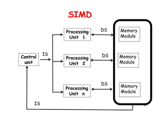
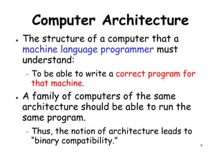
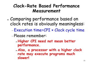
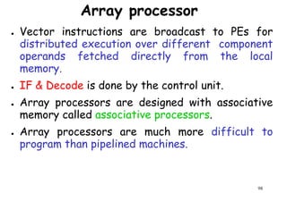
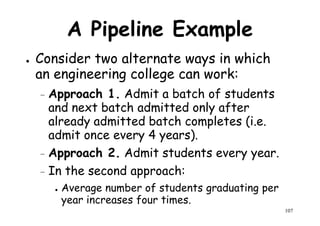
97. Array processor
● Synchronous parallel computer with multiple
arithmetic logic units [Same function at same
time] .
● By replication of ALU system can achieve
spatial parallelism.
● An appropriate data routing mechanism must
be establish among the PE’s.
Scalar & control type instructions are directly
97
● Scalar & control type instructions are directly
executed in control unit.
● Each PE consist of one ALU with register &
local memory.

98. Array processor
● Vector instructions are broadcast to PEs for
distributed execution over different component
operands fetched directly from the local
memory.memory.
● IF & Decode is done by the control unit.
● Array processors are designed with associative
memory called associative processors.
● Array processors are much more difficult to
98
● Array processors are much more difficult to
program than pipelined machines.

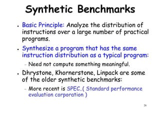
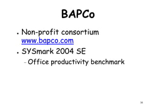
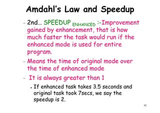
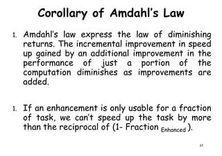
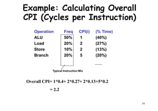
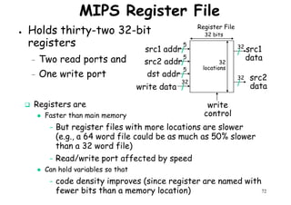
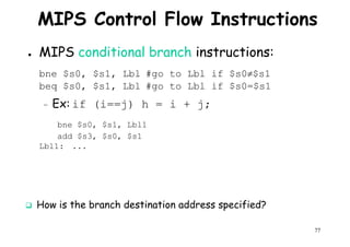
99. Control
Processor
Control
Memory
I/O
Control Unit P: Processor
M: Memory
Data Bus
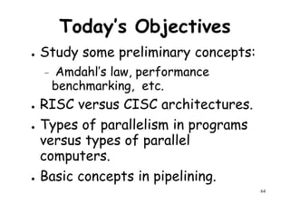
Scalar Processing
Duplicate Hardware PerformsDuplicate Hardware Performs
Multiple Tasks At OnceMultiple Tasks At Once
PP
M
P
MM
Array
Processing
. . . . .
PE1
PE 2
PE n
Control
99
Inter-PE connection network
[Data routing]
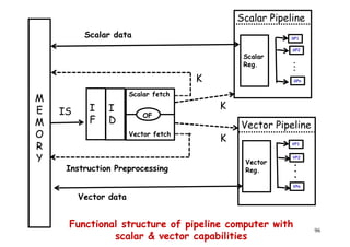
Functional structure of SIMD array processor with
concurrent scalar processing in control unit

100. Multiprocessor Systems
● Multiprocessor system leads to improving
throughput, reliability, &flexibility.
The enter system must be control by a● The enter system must be control by a
single integrated OS providing interaction
between processor & their programs at
various level.
● Each processor has its own local memory &
i/o devices.
100
i/o devices.
● Inter-processor communication can be
done through shared memories or through
an interrupt network.

101. Multiprocessor Systems
● There are three different types of inter-
processor communications are :
– Time shared common bus– Time shared common bus
– Crossbar switch network.
– Multiport memories.
● Centralized computing system, in which all
H/W & S/W resource are housed in the
same computing center with negligible
101
same computing center with negligible
communication delays among subsystems.
● Loosely coupled & tightly coupled.

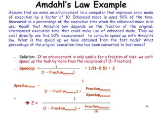
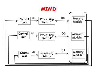
102. Memory
module 1
Memory
module 2
..
Input-output
Interconnection
Network
Interprocessor-memory
Connection network
[Bus , crossbar or multiport]
. . . . . .
I/O channels
Memory
module n
..
..
..
Shared Memory Inter-
processor
interrupt
P 1
LM1
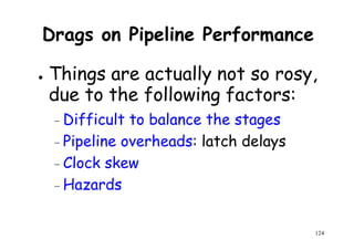
P 2 LM2
. . . .
102
interrupt
network
P n LM n
Functional design of an MIMD multiprocessor system

103. Parallel Execution of Programs
● Parallel execution of a program can be
done in one or more of following ways:
Instruction-level (Fine grained): individual– Instruction-level (Fine grained): individual
instructions on any one thread are executed
parallely.
● Parallel execution across a sequence of
instructions (block) -- could be a loop, a
conditional, or some other sequence of starts.
Thread-level (Medium grained): different
103
– Thread-level (Medium grained): different
threads of a process are executed parallely.
– Process-level (Coarse grained): different
processes can be executed parallely.

104. Exploitation of Instruction-Level
Parallelism
● ILP can be exploited by deploying several
available techniques:available techniques:
– Temporal parallelism (Overlapped execution):
● Pipelining
– Spatial Parallelism:
● Vector processing (single instruction multiple
data SIMD)
104
data SIMD)
● Superscalar execution (Multiple instructions
that use multiple data MIMD)

105. ILP Exploitation Through
Pipelining
105

106. Pipelining
● Pipelining incorporates the
concept of overlapped execution:concept of overlapped execution:
– Used in many everyday applications
without our notice.
● Has proved to be a very popular
and successful way to exploit ILP:
106
and successful way to exploit ILP:
– Instruction pipes are being used in
almost all modern processors.

107. A Pipeline Example
● Consider two alternate ways in which
an engineering college can work:an engineering college can work:
– Approach 1. Admit a batch of students
and next batch admitted only after
already admitted batch completes (i.e.
admit once every 4 years).
– Approach 2. Admit students every year.
107
– Approach 2. Admit students every year.
– In the second approach:
● Average number of students graduating per
year increases four times.

108. Pipelining
First Year Second Year Third Year Fourth Year
First Year Second Year Third Year Fourth Year
First Year Second Year Third Year Fourth Year
108

109. IFetch Dcd Exec Mem WB
Time
Pipelined Execution
IFetch Dcd Exec Mem WB
IFetch Dcd Exec Mem WB
IFetch Dcd Exec Mem WB
IFetch Dcd Exec Mem WB
IFetch Dcd Exec Mem WB
109
IFetch Dcd Exec Mem WB
Program Flow

110. Advantages of Pipelining
● An n-stage pipeline:
– Can improve performance upto n times.– Can improve performance upto n times.
● Not much investment in hardware:
– No replication of hardware resources
necessary.
– The principle deployed is to keep the
units as busy as possible.
110
– The principle deployed is to keep the
units as busy as possible.
● Transparent to the programmers:
– Easy to use

111. Basic Pipelining Terminologies
● Pipeline cycle (or Processor cycle):
– The time required to move an instruction
one step further in the pipeline.one step further in the pipeline.
– Not to be confused with clock cycle.
● Synchronous pipeline:
– Pipeline cycle is constant (clock-driven).
Asynchronous pipeline:
111
● Asynchronous pipeline:
– Time for moving from stage to stage varies
– Handshaking communication between stages

112. Principle of linear pipelining
● Assembly lines, where items are assembled
continuously from separate part along a moving
conveyor belt.
Partition of assembly depends on factors like:-● Partition of assembly depends on factors like:-
– Quality of working units
– Desired processing speed
– Cost effectiveness
All assembly stations must have equal
112
● All assembly stations must have equal
processing.
● Lowest station becomes the bottleneck or
congestion.

113. Precedence relation
● A set of subtask { T1,T2,……,Tn} for a given
task T ,that some task Tj can not start until
some earlier task Ti ,where (i<j)finishes.i ,
● Pipeline consists of cascade of processing
stages.
● Stages are combinational circuits over data
stream flowing through pipe.
Stages are separated by high speed interface
113
● Stages are separated by high speed interface
latches (Holding intermediate results between
stages.)
● Control must be under a common clock.

114. Synchronous Pipeline
- Transfers between stages are simultaneous.
- One task or operation enters the pipeline
S1 S2 Sk
LL LLL
Input Output
- One task or operation enters the pipeline
per cycle.
114
dτ τm
Clock

115. Asynchronous Pipeline
- Transfers performed when individual stages are
ready.
- Handshaking protocol between processors.
S1 S2 Sk
Output
Ready
Ack
Ready
Ack
Ready
Ack
Ready
Ack
Input
- Handshaking protocol between processors.
- Different amounts of delay may be experienced at
115
- Different amounts of delay may be experienced at
different stages.
- Can display variable throughput rate.

116. A Few Pipeline Concepts
Si Si+1Si Si+1
τ τm d
Pipeline cycle : τ
Latch delay : d
116
Latch delay : d
τ = max {τm } + d
Pipeline frequency : f
f = 1 / τ

117. Example on Clock period
● Suppose the time delays of the 4 stages are
τ1=60ns,τ2 = 50ns, τ3 = 90ns, τ4 = 80ns & the
interface latch has a delay of τl = 10ns. What is
the value of pipeline cycle time ?the value of pipeline cycle time ?
● Hence the cycle time of this pipeline can be
granted to be like :- τ = 90 + 10 =100ns
● Clock frequency of the pipeline (f) =1/100 =10 Mhz
● If it is non-pipeline then = 60+50+90+80 = 280ns
117
● If it is non-pipeline then = 60+50+90+80 = 280ns
τ = max {τm } + d

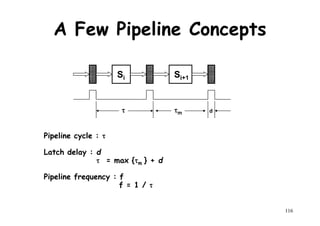
118. Ideal Pipeline Speedup
● k-stage pipeline processes n tasks in k + (n-1)
clock cycles:clock cycles:
– k cycles for the first task and n-1 cycles for the
remaining n-1 tasks.
● Total time to process n tasks
● Tk = [ k + (n-1)] τ
For the non-pipelined processor
118
● For the non-pipelined processor
T1 = n k τ

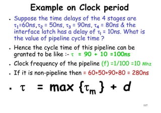
119. Pipeline Speedup Expression
Speedup=
● Maximum speedup = Sk K ,for n >> K
Sk =
T1
Tk
=
n k τ
[ k + (n-1)] τ
=
n k
k + (n-1)
119
● Observe that the memory bandwidth
must increase by a factor of Sk:
– Otherwise, the processor would stall waiting for
data to arrive from memory.

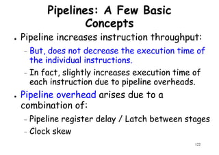
120. Efficiency of pipeline
● The percentage of busy time-space span over
the total time span.
– n:- no. of task or instruction– n:- no. of task or instruction
– k:- no. of pipeline stages
– τ:- clock period of pipeline
● Hence pipeline efficiency can be defined by:-
n * k * τ
η =
n
=
120
n * k * τ
K [ k*τ +(n-1) τ ]
η =
n
k+(n-1)
=

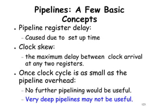
121. Throughput of pipeline
● Number of result task that can be completed
by a pipeline per unit time.
W =
n
=
n
=
η
● Idle case w = 1/τ = f when η =1.
W =
n
k*τ+(n-1)τ
=
n
[k+(n-1)]τ
=
η
τ
121
Idle case w = 1/τ = f when η =1.
● Maximum throughput = frequency of linear
pipeline

122. Pipelines: A Few Basic
Concepts
● Pipeline increases instruction throughput:
– But, does not decrease the execution time of– But, does not decrease the execution time of
the individual instructions.
– In fact, slightly increases execution time of
each instruction due to pipeline overheads.
● Pipeline overhead arises due to a
combination of:
122
combination of:
– Pipeline register delay / Latch between stages
– Clock skew

123. Pipelines: A Few Basic
Concepts
● Pipeline register delay:
– Caused due to set up time– Caused due to set up time
● Clock skew:
– the maximum delay between clock arrival
at any two registers.
● Once clock cycle is as small as the
123
● Once clock cycle is as small as the
pipeline overhead:
– No further pipelining would be useful.
– Very deep pipelines may not be useful.

124. Drags on Pipeline Performance
● Things are actually not so rosy,
due to the following factors:
Things are actually not so rosy,
due to the following factors:
– Difficult to balance the stages
– Pipeline overheads: latch delays
– Clock skew
124
– Clock skew
– Hazards

125. Exercise
● Consider an unpipelined processor:
– Takes 4 cycles for ALU and other operations– Takes 4 cycles for ALU and other operations
– 5 cycles for memory operations.
– Assume the relative frequencies:
● ALU and other=60%,
● memory operations=40%
– Cycle time =1ns
Compute speedup due to pipelining:
125
● Compute speedup due to pipelining:
– Ignore effects of branching.
– Assume pipeline overhead = 0.2ns

126. Solution
● Average instruction execution time for
large number of instructions:large number of instructions:
– unpipelined= 1ns * (60%*4+ 40%*5) =4.4ns
– Pipelined=1 + 0.2 = 1.2ns
● Speedup=4.4/1.2=3.7 times
126

127. Pipeline Hazards
● Hazards can result in incorrect
operations:
– Structural hazards: Two instructions– Structural hazards: Two instructions
requiring the same hardware unit at same
time.
– Data hazards: Instruction depends on result
of a prior instruction that is still in pipeline
● Data dependency
Control hazards: Caused by delay in decisions
127
Data dependency
– Control hazards: Caused by delay in decisions
about changes in control flow (branches and
jumps).
● Control dependency

128. Pipeline Interlock
● Pipeline interlock:
– Resolving of pipeline hazards through– Resolving of pipeline hazards through
hardware mechanisms.
● Interlock hardware detects all
hazards:
– Stalls appropriate stages of the
128
– Stalls appropriate stages of the
pipeline to resolve hazards.

129. MIPS
● MIPS architecture:
– First publicly known implementations of– First publicly known implementations of
RISC architectures
– Grew out of research at Stanford
University
● MIPS computer system founded in 1984:
R2000 introduced in 1986.
129
– R2000 introduced in 1986.
– Licensed the designs rather than selling
the design.

130. MIPS
cont…
● MIPS: Microprocessor Without
Interlocked Pipeline StagesInterlocked Pipeline Stages
● Operates on 64bit data
● 32 64bit registers
● 2 128KB high speed cache
Constant 32bit instruction length
130
● Constant 32bit instruction length
● Initial MIPS processors achieved
1instr/cycle (CPI =1)

131. MIPS Pipelining Stages
● 5 stages of MIPS Pipeline:
– IF Stage:
Needs access to the Memory to load the instruction.● Needs access to the Memory to load the instruction.
● Needs a adder to update the PC.
– ID Stage:
● Needs access to the Register File in reading operand.
● Needs an adder (to compute the potential branch target).
– EX Stage:
Needs an ALU.
131
● Needs an ALU.
– MEM Stage:
● Needs access to the Memory.
– WB Stage:
● Needs access to the Register File in writing.

132. Further MIPS Enhancements
cont…
● MIPS could achieve CPI of 1, to improve
performance further, two possibilities:performance further, two possibilities:
– Superscalar
– Superpipelined
● Superscalar:
– Replicate each pipeline stage so that two or
more instructions can proceed simultaneously.
132
more instructions can proceed simultaneously.
● Superpipeline:
– Split pipeline stages into further stages.

133. Summary
● RISC architecture style saves chip area
that is used to support more registers
and cache:and cache:
– Also instruction pipelining is facilitated due
to small and uniform sized instructions.
● Three main types of parallelism in a
program:
Instruction-level
133
– Instruction-level
– Thread-level
– Process-level

134. Summary
Cont…
● Two main types of parallel computers:
– SIMD
MIMD– MIMD
● Instruction pipelines are found in almost all
modern processors:
– Exploits instruction-level parallelism
– Transparent to the programmers
134
– Transparent to the programmers
● Hazards can slowdown a pipeline:
– In the next lecture, we shall examine hazards in
more detail and available ways to resolve hazards.

135. References
[1]J.L. Hennessy & D.A. Patterson,
“Computer Architecture: A Quantitative“Computer Architecture: A Quantitative
Approach”. Morgan Kaufmann Publishers,
3rd Edition, 2003
[2]John Paul Shen and Mikko Lipasti,
“Modern Processor Design,” Tata Mc-
Graw-Hill, 2005
135
Graw-Hill, 2005