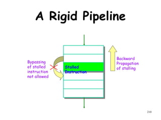
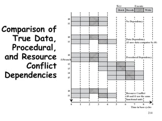
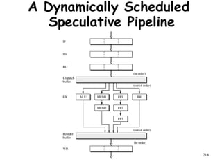
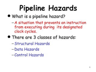
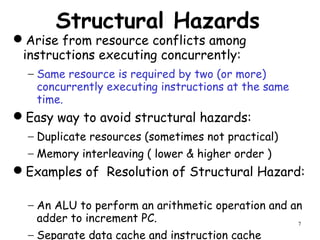
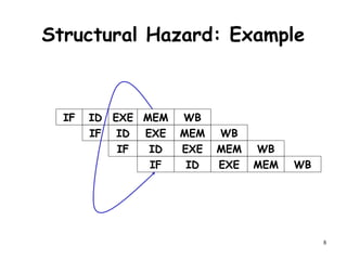
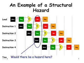
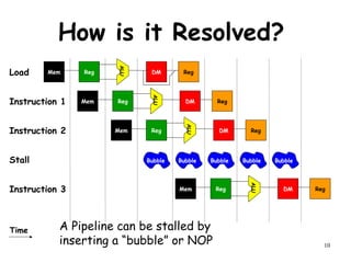
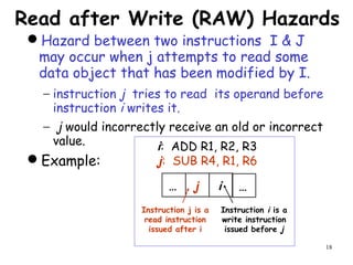
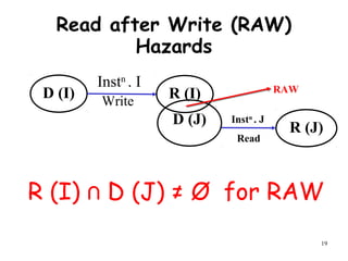
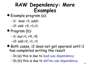
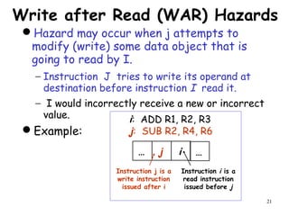
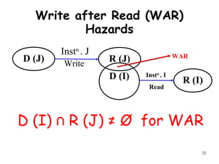
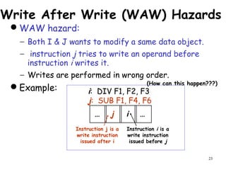
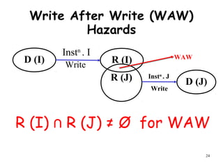
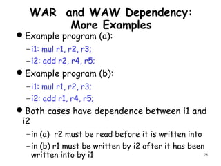
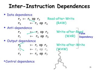
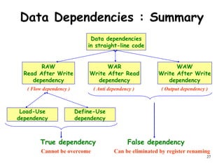
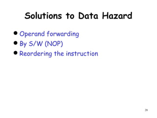
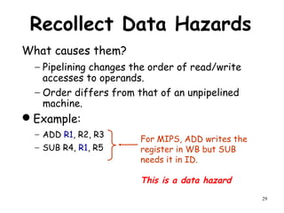
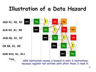
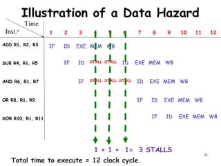
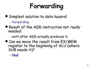
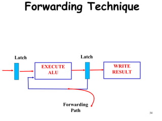
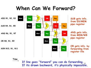
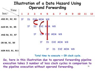
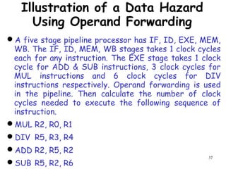
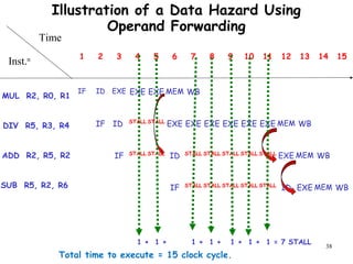
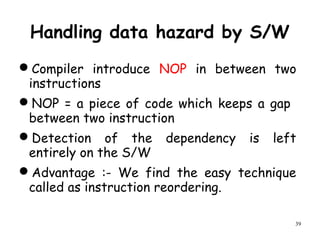
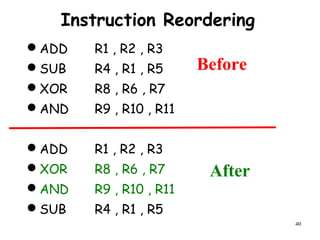
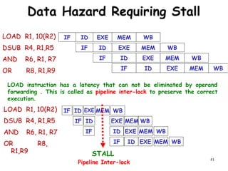
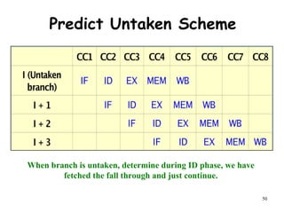
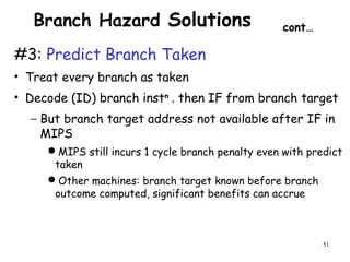
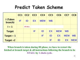
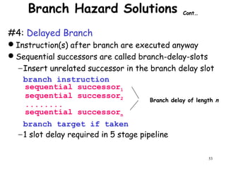
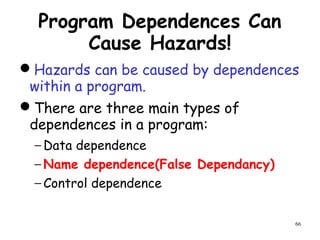
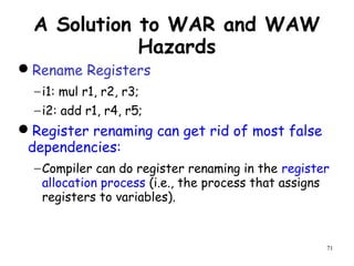
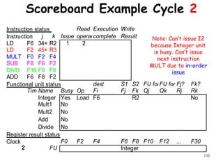
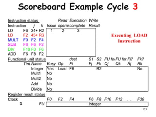
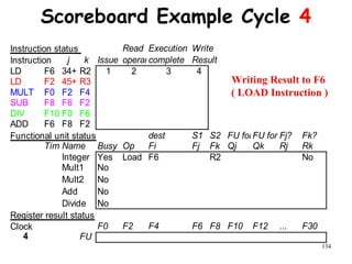
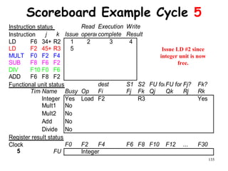
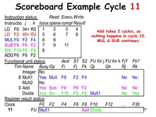
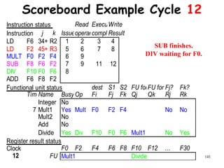
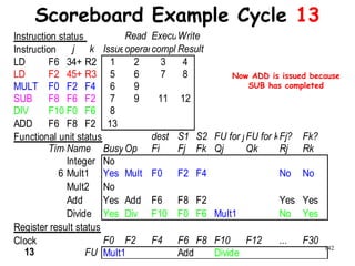
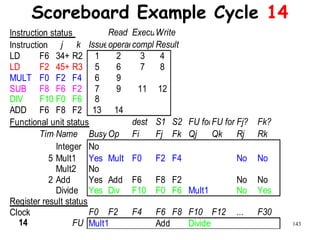
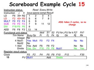
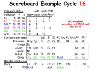
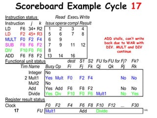
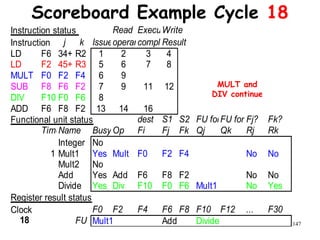
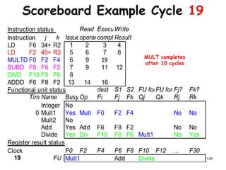
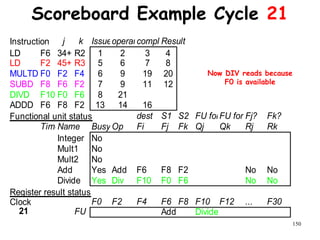
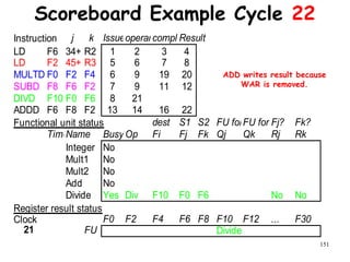
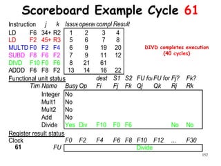
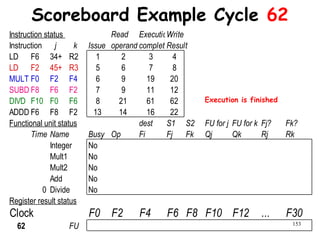
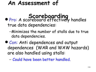
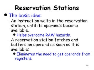
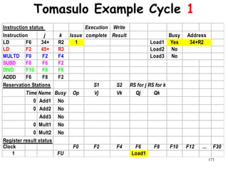
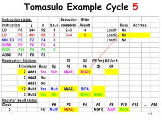
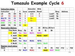
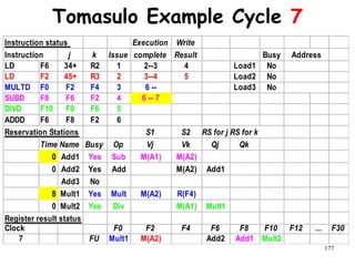
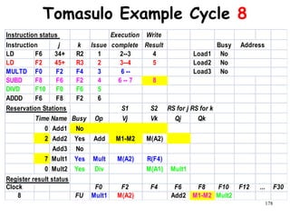
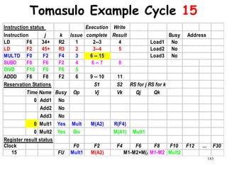
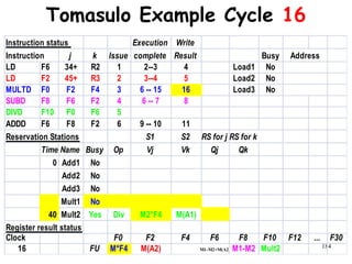
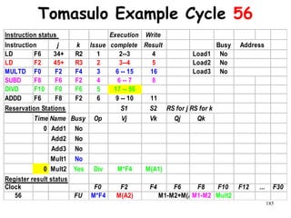
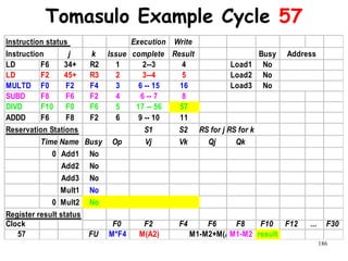
The document discusses pipeline hazards in computer architecture and their resolution mechanisms. There are three types of hazards: structural hazards which occur due to resource conflicts, data hazards which occur when an instruction depends on data from a prior instruction, and control hazards which occur due to conditional branch instructions. Data hazards include read after write (RAW), write after read (WAR), and write after write (WAW) hazards. Forwarding is a common technique to resolve data hazards by passing results directly from one pipeline stage to another as needed. Stalls can also resolve hazards by inserting no-operation instructions but reduce pipeline efficiency.


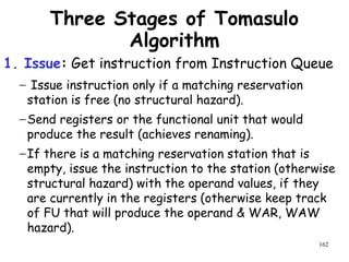
![91
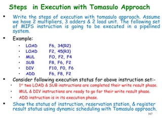
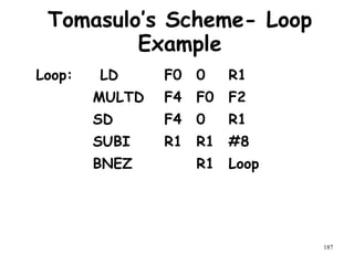
Loop-level Parallelism
It may be possible to execute
different iterations of a loop in
parallel.
Example:
− For(i=0;i<1000;i++){
− a[i]=a[i]+b[i];
− b[i]=b[i]*2;
− }](https://image.slidesharecdn.com/module2-190326205728/85/High-Performance-Computer-Architecture-88-320.jpg)
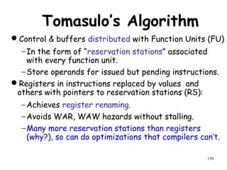
![93
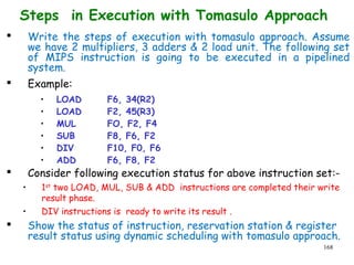
Loop-level Dependence
Example:
− For(i=0;i<1000;i++){
− a[i+1]=b[i]+c[i]
− b[i+1]=a[i+1]+d[i];
− }
Loop-carried dependence from one iteration to
the preceding iteration.
Also, loop-independent dependence on account of
a[i+1]](https://image.slidesharecdn.com/module2-190326205728/85/High-Performance-Computer-Architecture-90-320.jpg)
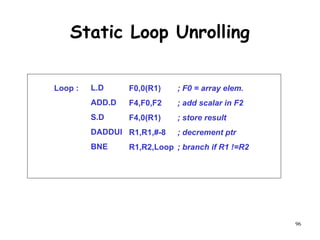
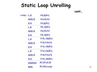
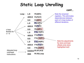
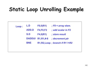
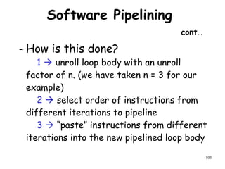
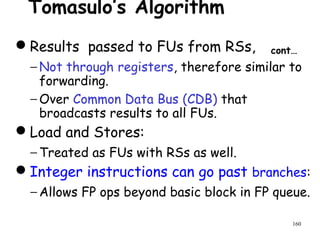
![95
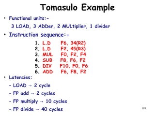
Static Loop Unrolling
- A high proportion of loop instructions are
loop management instructions.
- Eliminating this overhead can significantly
increase the performance of the loop.
- for(i=1000;i>0;i--)
- {
- a[i]=a[i]+c;
- }](https://image.slidesharecdn.com/module2-190326205728/85/High-Performance-Computer-Architecture-92-320.jpg)
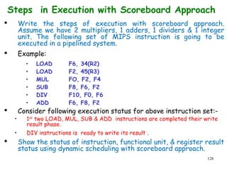
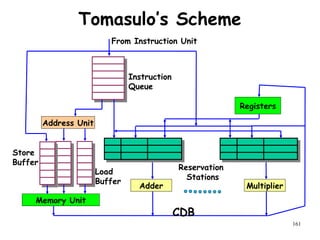
![108
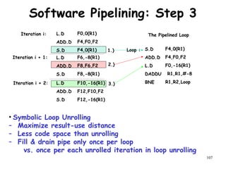
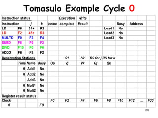
Software Pipelining: Step 4
S.D
ADD.D
L.D
DADDUI
BNE
Loop : F4,16(R1)
F4,F0,F2
F0,0(R1)
R1,R1,#-8
R1,R2,Loop
; M[ i ]
; M[ i – 1 ]
; M[ i – 2 ]
Instructions to fill “software pipeline”
Pipelined Loop Body
Preheader
Postheader
Instructions to drain “software pipeline”](https://image.slidesharecdn.com/module2-190326205728/85/High-Performance-Computer-Architecture-105-320.jpg)
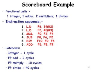


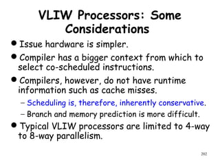
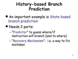
![192
A Practice Problem on
Dependence Analysis
Identify all dependences in the following
code.
Transform the code to eliminate the
dependences.
for(i=1;i<1000;i++){
y[i]=x[i]/c;
x[i]=x[i]+c;
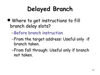
z[i]=y[i]+c;
y[i]=c-y[i];
}](https://image.slidesharecdn.com/module2-190326205728/85/High-Performance-Computer-Architecture-189-320.jpg)
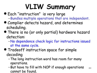
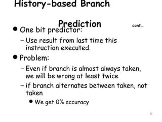
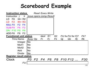
![193
Transformed Code Without
Dependence
for(i=1;i<1000;i++){
t[i]=x[i]/c;
x[i]=x[i]+c;
z[i]=t[i]+c;
y[i]=c-t[i];
}](https://image.slidesharecdn.com/module2-190326205728/85/High-Performance-Computer-Architecture-190-320.jpg)