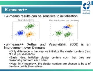
• 𝐾-means resultscan be sensitive to initialization
• 𝐾-means++ (Arthur and Vassilvitskii, 2006) is an
improvement over 𝐾-means
• Only difference is the way we initialize the cluster centers (rest
of it is just 𝐾-means)
• Basic idea: Initialize cluster centers such that they are
reasonably far from each other
• Note: In 𝐾-means++, the cluster centers are chosen to be 𝐾 of
the data points themselves
K-means++
Poor initialization: bad clustering
Desired clustering
3.
• K-means++ worksas follows
• Choose the first cluster mean uniformly randomly to be one of
the data points
• The subsequent 𝐾−1 cluster means are chosen as follows
• (1) For each unselected point 𝒙, compute its smallest distance 𝐷(𝒙)
from already initialized means
• (2) Select the next cluster mean uniformly at random to be one of the
unselected points based on probability prop. to 𝐷(𝒙) i.e.,
(𝒙)
∑ (𝒙)
∈𝒳
• (3) Repeat 1 and 2 until the 𝐾−1 cluster means are initialized
• Now run standard K-means with these initial cluster means
• K-means++ initialization scheme sort of ensures that the
initial cluster means are located in different clusters
K-means++
Thus farthest points are
most likely to be selected
as cluster means
4.
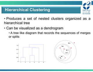
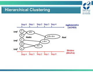
• Produces aset of nested clusters organized as a
hierarchical tree
• Can be visualized as a dendrogram
• A tree like diagram that records the sequences of merges
or splits
Hierarchical Clustering
1 3 2 5 4 6
0
0.05
0.1
0.15
0.2
1
2
3
4
5
6
1
2
3 4
5
5.
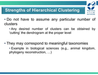
• Do nothave to assume any particular number of
clusters
• Any desired number of clusters can be obtained by
‘cutting’ the dendrogram at the proper level
• They may correspond to meaningful taxonomies
• Example in biological sciences (e.g., animal kingdom,
phylogeny reconstruction, …)
Strengths of Hierarchical Clustering
6.
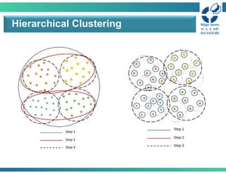
• Two maintypes of hierarchical clustering
• Agglomerative:
• Start with the points as individual clusters
• At each step, merge the closest pair of clusters until only one
cluster (or 𝑘 clusters) left
• Divisive:
• Start with one, all-inclusive cluster
• At each step, split a cluster until each cluster contains an
individual point (or there are 𝑘 clusters)
• Traditional hierarchical algorithms use a similarity or
distance matrix
• Merge or split one cluster at a time
Hierarchical Clustering
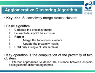
• Key Idea:Successively merge closest clusters
• Basic algorithm
1. Compute the proximity matrix
2. Let each data point be a cluster
3. Repeat
4. Merge the two closest clusters
5. Update the proximity matrix
6. Until only a single cluster remains
• Key operation is the computation of the proximity of two
clusters
• Different approaches to define the distance between clusters
distinguish the different algorithms
Agglomerative Clustering Algorithm
10.
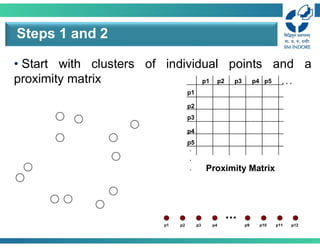
• Start withclusters of individual points and a
proximity matrix
Steps 1 and 2
p1
p3
p5
p4
p2
p1 p2 p3 p4 p5 . . .
.
.
. Proximity Matrix
11.
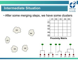
• After somemerging steps, we have some clusters
Intermediate Situation
C1
C4
C2 C5
C3
C2
C1
C1
C3
C5
C4
C2
C3 C4 C5
Proximity Matrix
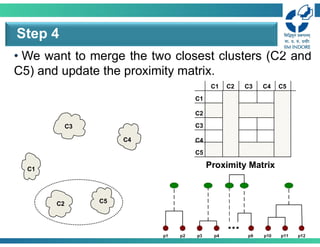
12.
• We wantto merge the two closest clusters (C2 and
C5) and update the proximity matrix.
Step 4
C1
C4
C2 C5
C3
C2
C1
C1
C3
C5
C4
C2
C3 C4 C5
Proximity Matrix
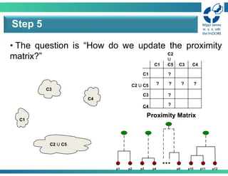
13.
• The questionis “How do we update the proximity
matrix?”
Step 5
C1
C4
C2 U C5
C3
? ? ? ?
?
?
?
C2
U
C5
C1
C1
C3
C4
C2 U C5
C3 C4
Proximity Matrix
14.
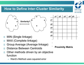
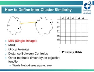
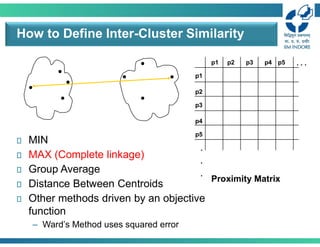
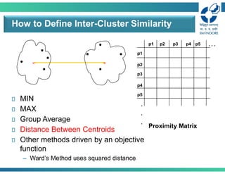
How to DefineInter-Cluster Similarity
p1
p3
p5
p4
p2
p1 p2 p3 p4 p5 . . .
.
.
.
Similarity?
MIN (Single linkage)
MAX (Complete linkage)
Group Average (Average linkage)
Distance Between Centroids
Other methods driven by an objective
function
– Ward’s Method uses squared error
Proximity Matrix
15.
How to DefineInter-Cluster Similarity
p1
p3
p5
p4
p2
p1 p2 p3 p4 p5 . . .
.
.
.
Proximity Matrix
MIN (Single linkage)
MAX
Group Average
Distance Between Centroids
Other methods driven by an objective
function
– Ward’s Method uses squared error
16.
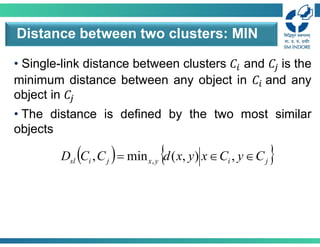
• Single-link distancebetween clusters 𝐶 and 𝐶 is the
minimum distance between any object in 𝐶 and any
object in 𝐶
• The distance is defined by the two most similar
objects
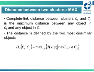
Distance between two clusters: MIN
j
i
y
x
j
i
sl C
y
C
x
y
x
d
C
C
D
,
)
,
(
min
, ,
17.
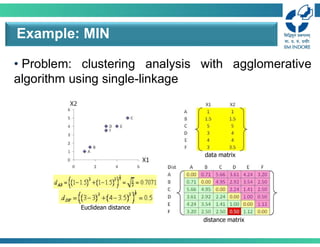
• Problem: clusteringanalysis with agglomerative
algorithm using single-linkage
Example: MIN
data matrix
distance matrix
Euclidean distance
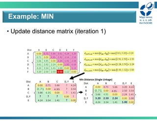
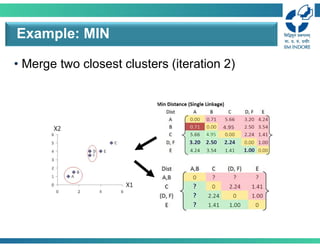
18.
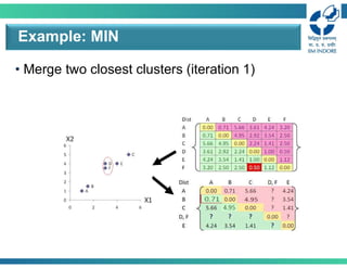
• Merge twoclosest clusters (iteration 1)
Example: MIN
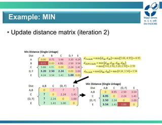
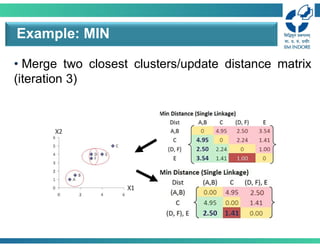
• Merge twoclosest clusters/update distance matrix
(iteration 3)
Example: MIN
23.
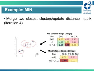
• Merge twoclosest clusters/update distance matrix
(iteration 4)
Example: MIN
24.
• Final result(meeting termination condition)
Example: MIN
25.
How to DefineInter-Cluster Similarity
p1
p3
p5
p4
p2
p1 p2 p3 p4 p5 . . .
.
.
.
Proximity Matrix
MIN
MAX (Complete linkage)
Group Average
Distance Between Centroids
Other methods driven by an objective
function
– Ward’s Method uses squared error
26.
• Complete-link distancebetween clusters 𝐶 and 𝐶
is the maximum distance between any object in
𝐶 and any object in 𝐶
• The distance is defined by the two most dissimilar
objects
Distance between two clusters: MAX
j
i
y
x
j
i
cl C
y
C
x
y
x
d
C
C
D
,
)
,
(
max
, ,
27.
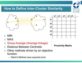
How to DefineInter-Cluster Similarity
p1
p3
p5
p4
p2
p1 p2 p3 p4 p5 . . .
.
.
.
Proximity Matrix
MIN
MAX
Group Average (Average linkage)
Distance Between Centroids
Other methods driven by an objective
function
– Ward’s Method uses squared error
28.
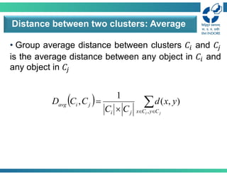
• Group averagedistance between clusters 𝐶 and 𝐶
is the average distance between any object in 𝐶 and
any object in 𝐶
Distance between two clusters: Average
j
i C
y
C
x
j
i
j
i
avg y
x
d
C
C
C
C
D
,
)
,
(
1
,
29.
How to DefineInter-Cluster Similarity
p1
p3
p5
p4
p2
p1 p2 p3 p4 p5 . . .
.
.
.
Proximity Matrix
MIN
MAX
Group Average
Distance Between Centroids
Other methods driven by an objective
function
– Ward’s Method uses squared distance
30.
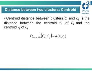
• Centroid distancebetween clusters 𝐶 and 𝐶 is the
distance between the centroid 𝑟 of 𝐶 and the
centroid 𝑟 of 𝐶
Distance between two clusters: Centroid
)
,
(
, j
i
j
i
centroids r
r
d
C
C
D
31.
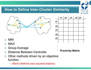
How to DefineInter-Cluster Similarity
p1
p3
p5
p4
p2
p1 p2 p3 p4 p5 . . .
.
.
.
Proximity Matrix
MIN
MAX
Group Average
Distance Between Centroids
Other methods driven by an objective
function
– Ward’s Method uses squared distance
+
32.
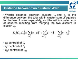
• Ward’s distancebetween clusters 𝐶 and 𝐶 is the
difference between the total within cluster sum of squares
for the two clusters separately, and the within cluster sum
of squares resulting from merging the two clusters in
cluster 𝐶
• 𝑟 : centroid of 𝐶
• 𝑟 : centroid of 𝐶
• 𝑟 : centroid of 𝐶
Distance between two clusters: Ward
ij
j
i C
x
ij
C
x
j
C
x
i
j
i
w r
x
r
x
r
x
C
C
D
2
2
2
,
33.
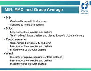
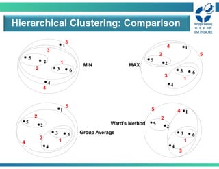
• MIN
• Canhandle non-elliptical shapes
• Sensitive to noise and outliers
• MAX
• Less susceptible to noise and outliers
• Tends to break large clusters and biased towards globular clusters
• Group average
• Compromise between MIN and MAX
• Less susceptible to noise and outliers
• Biased towards globular clusters
• Ward
• Similar to group average and centroid distance
• Less susceptible to noise and outliers
• Biased towards globular clusters
MIN, MAX, and Group Average
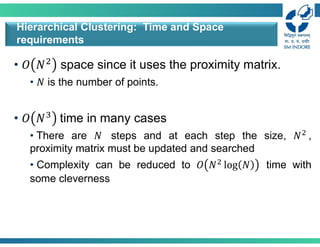
• 𝑂 𝑁space since it uses the proximity matrix.
• 𝑁 is the number of points.
• 𝑂 𝑁 time in many cases
• There are 𝑁 steps and at each step the size, 𝑁 ,
proximity matrix must be updated and searched
• Complexity can be reduced to 𝑂 𝑁 log 𝑁 time with
some cleverness
Hierarchical Clustering: Time and Space
requirements
36.
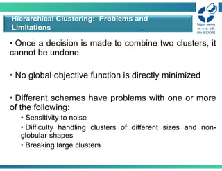
• Once adecision is made to combine two clusters, it
cannot be undone
• No global objective function is directly minimized
• Different schemes have problems with one or more
of the following:
• Sensitivity to noise
• Difficulty handling clusters of different sizes and non-
globular shapes
• Breaking large clusters
Hierarchical Clustering: Problems and
Limitations
37.
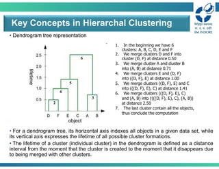
• Dendrogram treerepresentation
• For a dendrogram tree, its horizontal axis indexes all objects in a given data set, while
its vertical axis expresses the lifetime of all possible cluster formations.
• The lifetime of a cluster (individual cluster) in the dendrogram is defined as a distance
interval from the moment that the cluster is created to the moment that it disappears due
to being merged with other clusters.
Key Concepts in Hierarchal Clustering
1. In the beginning we have 6
clusters: A, B, C, D, E and F
2. We merge clusters D and F into
cluster (D, F) at distance 0.50
3. We merge cluster A and cluster B
into (A, B) at distance 0.71
4. We merge clusters E and (D, F)
into ((D, F), E) at distance 1.00
5. We merge clusters ((D, F), E) and C
into (((D, F), E), C) at distance 1.41
6. We merge clusters (((D, F), E), C)
and (A, B) into ((((D, F), E), C), (A, B))
at distance 2.50
7. The last cluster contain all the objects,
thus conclude the computation
2
3
4
5
6
object
lifetime
38.
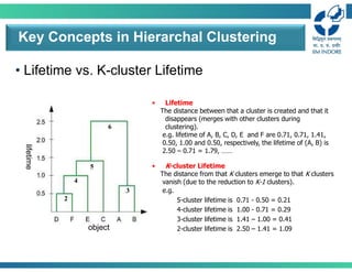
• Lifetime vs.K-cluster Lifetime
Key Concepts in Hierarchal Clustering
2
3
4
5
6
object
lifetime
• Lifetime
The distance between that a cluster is created and that it
disappears (merges with other clusters during
clustering).
e.g. lifetime of A, B, C, D, E and F are 0.71, 0.71, 1.41,
0.50, 1.00 and 0.50, respectively, the lifetime of (A, B) is
2.50 – 0.71 = 1.79, ……
• K-cluster Lifetime
The distance from that K clusters emerge to that K clusters
vanish (due to the reduction to K-1 clusters).
e.g.
5-cluster lifetime is 0.71 - 0.50 = 0.21
4-cluster lifetime is 1.00 - 0.71 = 0.29
3-cluster lifetime is 1.41 – 1.00 = 0.41
2-cluster lifetime is 2.50 – 1.41 = 1.09
39.
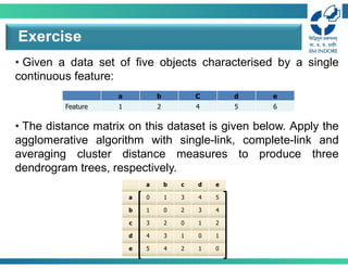
• Given adata set of five objects characterised by a single
continuous feature:
• The distance matrix on this dataset is given below. Apply the
agglomerative algorithm with single-link, complete-link and
averaging cluster distance measures to produce three
dendrogram trees, respectively.
Exercise
e
d
C
b
a
6
5
4
2
1
Feature
e
d
c
b
a
5
4
3
1
0
a
4
3
2
0
1
b
2
1
0
2
3
c
1
0
1
3
4
d
0
1
2
4
5
e
40.
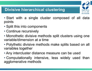
• Start witha single cluster composed of all data
points
• Split this into components
• Continue recursively
• Monothetic divisive methods split clusters using one
variable/dimension at a time
• Polythetic divisive methods make splits based on all
variables together
• Any intercluster distance measure can be used
• Computationally intensive, less widely used than
agglomerative methods
Divisive hierarchical clustering
41.
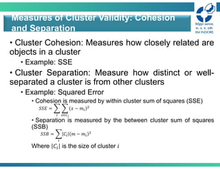
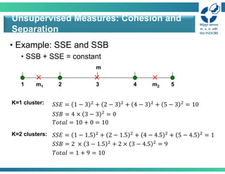
• Cluster Cohesion:Measures how closely related are
objects in a cluster
• Example: SSE
• Cluster Separation: Measure how distinct or well-
separated a cluster is from other clusters
• Example: Squared Error
• Cohesion is measured by within cluster sum of squares (SSE)
• Separation is measured by the between cluster sum of squares
(SSB)
Where 𝐶 is the size of cluster 𝑖
Measures of Cluster Validity: Cohesion
and Separation
𝑆𝑆𝐸 = 𝑥 − 𝑚
∈
𝑆𝑆𝐵 = 𝐶 𝑚 − 𝑚
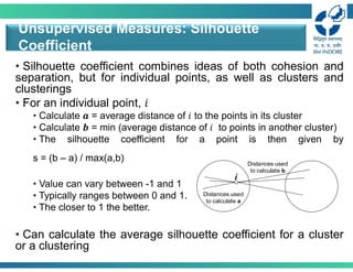
• Silhouette coefficientcombines ideas of both cohesion and
separation, but for individual points, as well as clusters and
clusterings
• For an individual point, 𝑖
• Calculate 𝒂 = average distance of 𝑖 to the points in its cluster
• Calculate 𝒃 = min (average distance of 𝑖 to points in another cluster)
• The silhouette coefficient for a point is then given by
s = (b – a) / max(a,b)
• Value can vary between -1 and 1
• Typically ranges between 0 and 1.
• The closer to 1 the better.
• Can calculate the average silhouette coefficient for a cluster
or a clustering
Unsupervised Measures: Silhouette
Coefficient
Distances used
to calculate a
i
Distances used
to calculate b
44.
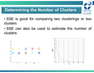
• SSE isgood for comparing two clusterings or two
clusters
• SSE can also be used to estimate the number of
clusters
Determining the Number of Clusters
2 5 10 15 20 25 30
0
1
2
3
4
5
6
7
8
9
10
K
SSE
5 10 15
-6
-4
-2
0
2
4
6